Suppose we create a large table in excel spreadsheet and it lists large amount of data. There are headers in the first row, and if we want to drag the scroll bar to view the bottom of table, the headers are hidden due to it lists on the top. So, in this case if we want to see the headers all the time, we need to freeze the first row to make it fixed and always displays on the top even we drag the scrollbar. On the other side, sometimes we need to freeze more rows, or columns, or even freeze row and column simultaneously. To implement this, we need to know the way to freeze row and columns. This article will introduce different ways to freeze row and columns with examples for you, you can’t miss it.
Table of Contents
Method 1: How to Freeze the First Row in Excel Spreadsheet
In most daily work, freeze the first row in table is frequently needed due to in most tables the first row lists the headers. So, people always want to see the headers on top no matter whether they drag the scrollbar to the end or not. See example below:
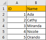
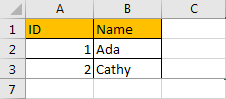
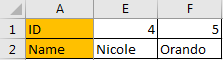
Suppose it lists a long list of ID and names. Header ID and Name are listed on the top. Now let’s freeze the first row.
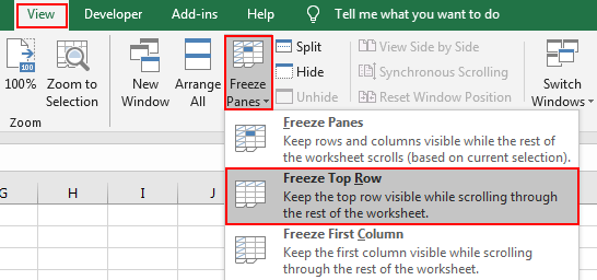
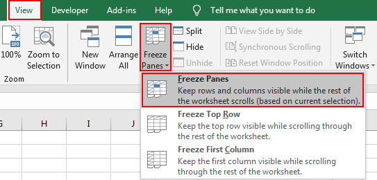
Step 1: Click View in the ribbon, then click Freeze Panes in Window group, then click the small triangle of Freeze Panes to load below three options, select the middle one ‘Freeze Top Row’.
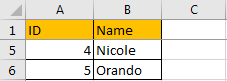
Step 2: After above operating. The first top row is fixed and always displayed on the top. Try to drag the scrollbar. You can see the header row is stayed on the top.
Method 2: How to Freeze Multiple Rows in Excel Spreadsheet
If you want to freeze the first three rows in excel, you can just select the first cell in the fourth row, then freeze the rows above the selected cell. See details below.
Step 1: Click A4 in the table.
Step 2: Click View in the ribbon, then click Freeze Panes in Window group, then click the small triangle of Freeze Panes to load below three options, select the first one ‘Freeze Panes’.
Step 3: Try to drag the scrollbar. Verify that top three rows are fixed.
Method 3: How to Freeze the First Column in Excel Spreadsheet
See screenshot below:
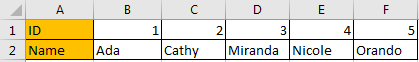
Now let’s freeze the first column. The way is similar with freeze the first row.
Step 1: Click View in the ribbon, then click Freeze Panes in Window group, then click the small triangle of Freeze Panes to load below three options, select the middle one ‘Freeze First Column’.
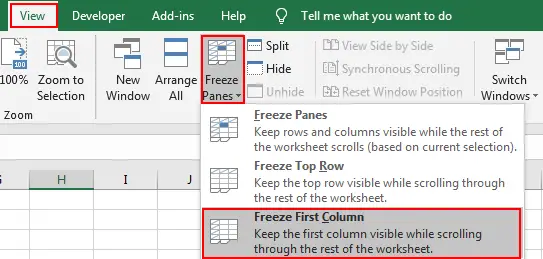
Step 2: Verify if it works well.
Obviously, it works.
Method 4: How to Freeze Row and Column in Excel Spreadsheet
If you want to just freeze the first row and column, just click on B2. Then click View->Freeze Panes->Freeze Panes in Window group.

Method 5: How to Freeze Rows and Columns in Excel Spreadsheet
If you want to freeze multiple rows and columns, refer to the description of Freeze Panes ‘Keep rows and column visible while the rest of the worksheet scrolls (based on current selection)’ we can know that we can select a cell to make it as the first cell outside of your fixed area. For example, if we want to freeze the top three rows and first two columns (row 4 is not fixed and column C is not fixed), we can click on C4, then repeat above steps to freeze panes.