This post will provide you with two different methods to lookup the next largest value in Excel: using a formula and using VBA code. While both methods achieve the same result, they differ in their implementation and can be used depending on your specific requirements.

1. Find the Next Largest Value Using Formula

If you want to get the next largest value in another column, you can use a combination of the INDEX function and the MATCH function to create an excel formula.

For example, if we used the VLOOKUP function to lookup the value 200, then it returns “103”, so it returns the value that is less than or equal to the lookup value. but if you want to return the next largest value in the range A2:A5, you can use the following formula:

=INDEX(A2:A5,MATCH(200,A2:A5)+1)

And if you want to find the next largest value in another column B2:B5, you just need to change the first argument of the INDEX function, use the range B2:B5 instead of A2:A5, the formula is as follwos:

=INDEX(B2:B5,MATCH(200,A2:A5)+1)

Let’s see how the above formula works:

=MATCH(200,A2:A5)+1

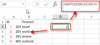
The MATCH function return the position of the lookup value 200 in the range A2:A5, if the MATCH function is not find the exact match, then it would return an approximate matched value(it should be less than or equalt to the lookup value) by default, so it returns 1.

To get the position of the next largest value, the position number returned by the match function need to add 1 again. so now we got the position of the next largest value in the range A2:A5. It returns 2.

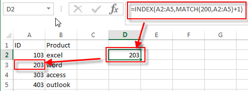
=INDEX(A2:A5,MATCH(200,A2:A5)+1)

=INDEX(B2:B5,MATCH(200,A2:A5)+1)

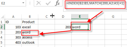
The INDEX function returns the value based on the given position that returned by the above MATCH function.

so if you used the Range A2:A5, then the above INDEX function returns the next largest value in the range A2:A5.

And if you used the Range B2:B5, then it returns the next largest value in the range B2:B5.

You can also use the following array formula to achieve the same result.

=INDEX(B2:B5,MATCH(TRUE,A2:A5>200,0))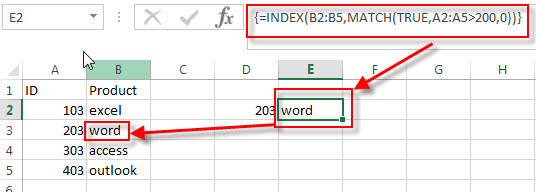

Note: when you enter the above array formula into a single cell, you should press Ctrl + Shift +Enter key.

2. Find the Next Largest Value with VBA Code (User Defined Function)

You can also create a User defined function with VBA code to find the next largest value in a given range of cells in Excel. Just do the following steps:

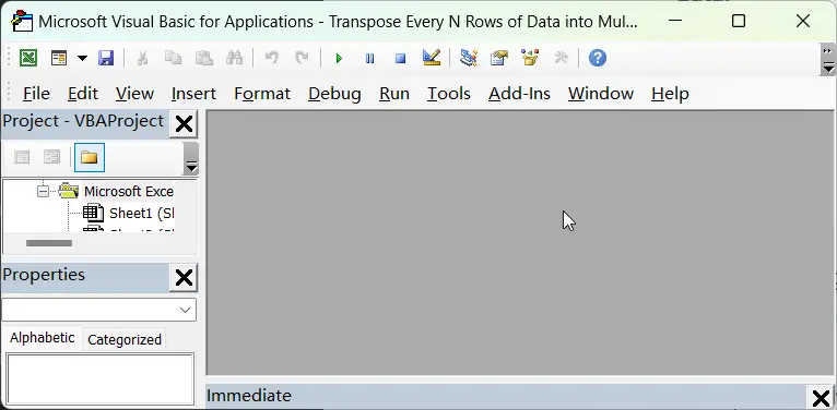
Step1: Open your Excel workbook and press “Alt + F11” to open the Visual Basic Editor.

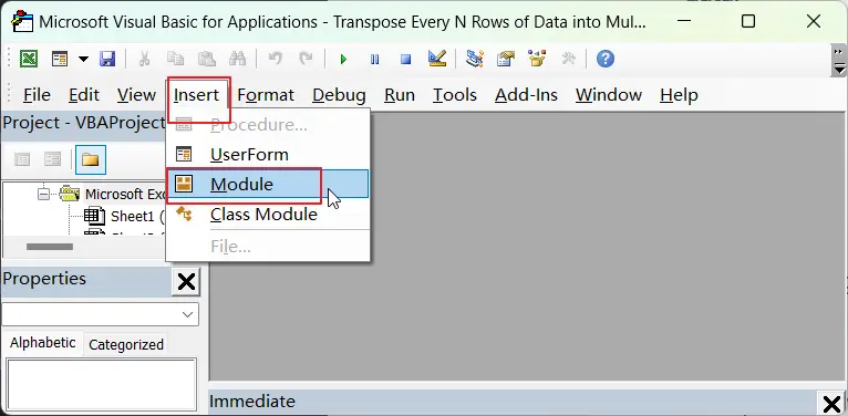
Step2: In the Editor, go to “Insert” > “Module” to create a new module.

Step3: Copy and paste the following code into the new module:

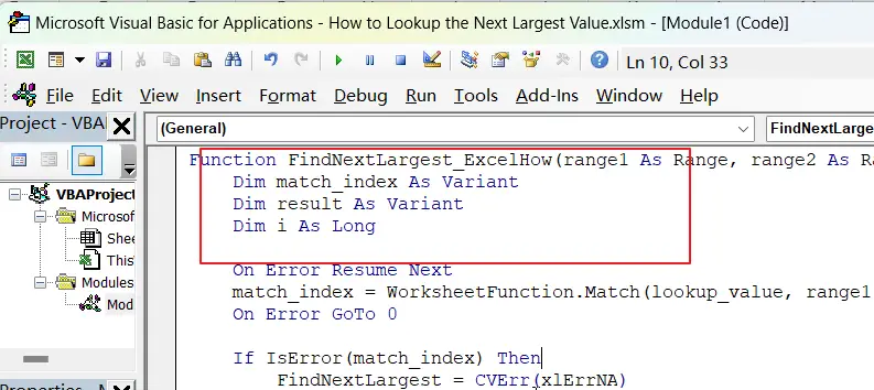
Function FindNextLargest_ExcelHow(range1 As Range, range2 As Range, lookup_value As Double) As Variant
    Dim match_index As Variant
    Dim result As Variant
    Dim i As Long
    
    On Error Resume Next
    match_index = WorksheetFunction.Match(lookup_value, range1, 0)
    On Error GoTo 0
    
    If IsError(match_index) Then
        FindNextLargest_ExcelHow = CVErr(xlErrNA)
    Else
        For i = match_index + 1 To range1.Cells.Count
            If range1.Cells(i).Value > lookup_value Then
                result = range2.Cells(i).Value
                Exit For
            End If
        Next i
        
        If IsEmpty(result) Then
            FindNextLargest_ExcelHow = CVErr(xlErrNA)
        Else
            FindNextLargest_ExcelHow = result
        End If
    End If
End Function

Step4: Save the module by going to “File” > “Save” and then close the Editor.

Step5: In your worksheet, select the cell where you want to display the next largest value. Type the following formula into the formula bar:

=FindNextLargest(A2:A5,B2:B5,200)

Note: you will need to replace the ranges A2:A5 and B2:B5 as you need.

Step6: this formula should return “word”, which is the next largest value in column A after 200.

3. Video: Find the Next Largest Value

This video will demonstrate how to lookup the next largest value using both a formula and VBA code.

4. Related Formulas

• Find the Relative Position in a Range or Table
  If you want to know the relative row position for all rows in an Excel Range (B3:D6), you can use a excel Array formula as follows:=ROW(B3:D6)- ROW(B3) + 1. You can also use another excel array formula to get the same result as follows:=ROW(B3:D6)-ROW(INDEX(B3:D6,1,1))+1…
• Reverse a List or Range
  If you want to reverse a list or range, you can use a combination of the INDEX function, the COUNTA function, the ROW function or ROWS function to create a new formula. you can use the following formula:=INDEX($A$2:$A$5,COUNTA($A$2:$A$5)-ROWS($C$2:C2)+1)…

5. Related Functions

• Excel INDEX function
  The Excel INDEX function returns a value from a table based on the index (row number and column number)The INDEX function is a build-in function in Microsoft Excel and it is categorized as a Lookup and Reference Function.The syntax of the INDEX function is as below:= INDEX (array, row_num,[column_num])…
• Excel MATCH function
  The Excel MATCH function search a value in an array and returns the position of that item.The syntax of the MATCH function is as below:= MATCH  (lookup_value, lookup_array, [match_type])….
• Excel VLOOKUP function
  The Excel VLOOKUP function lookup a value in the first column of the table and return the value in the same row based on index_num position.The syntax of the VLOOKUP function is as below:= VLOOKUP (lookup_value, table_array, column_index_num,[range_lookup])….