This post will guide you how to reverse order of rows in Excel. How do I flip data in rows with VBA Macro in Excel. Is there any simple way to reverse the order of some rows in Excel.

Reverse the Order of Rows

---

Assuming that you have a list of data in range A1:D2, and you want to reverse the order of rows in the selected range in Excel. You can use an Excel VBA Macro to achieve the result of reversing the order of all rows in range A1:D2. Just do the following steps:

#1 open your excel workbook and then click on “Visual Basic” command under DEVELOPER Tab, or just press “ALT+F11” shortcut.

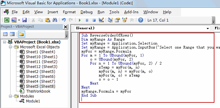
#2 then the “Visual Basic Editor” window will appear.

#3 click “Insert” ->”Module” to create a new module.

#4 paste the below VBA code  into the code window. Then clicking “Save” button.

Sub ReverseOrderOfRows()

    Set myRange = Application.Selection
    Set myRange = Application.InputBox("Select one Range that you want to reverse the order of rows:", , myRange.Address, Type:=8)
    myFor = myRange.Formula

    For m = 1 To UBound(myFor, 1)
        o = UBound(myFor, 2)
        For n = 1 To UBound(myFor, 2) / 2
            Temp = myFor(m, n)
            myFor(m, n) = myFor(m, o)
            myFor(m, o) = Temp
            o = o - 1
        Next
    Next
    myRange.Formula = myFor
End Sub

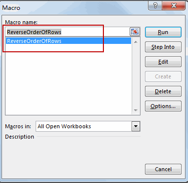
#5 back to the current worksheet, then run the above excel macro. Click Run button.

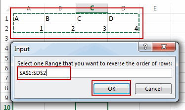
#6  Select one Range that you want to reverse the order of rows. Click OKbutton.

#7 Let’s see the result: