This post will guide you how to select cells that meet certain criteria in Excel. How do I find and select cells based on specific types of data in your worksheet in Excel.

• Select Cells That Meet one Criteria Using Go To Command
• Find Cells That Meet one Criteria Using Conditional Formatting

Select Cells That Meet one Criteria Using Go To Command

---

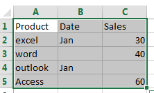
Assuming that you have a list of data in range A1:C5, and you want to select cells that contain specific types of data, such as: formulas, blanks, non-blanks, etc. How to do it. You can use the Go To command to quickly find and select all cells that meet your specific conditions.

For example, you need to select all blanks in the selected range of cell, just do the following steps:

#1 select the range of cells that you want to find for specific cells.

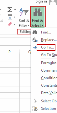
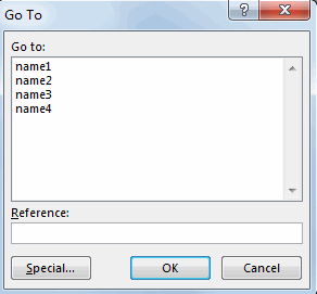
#2 go to HOME tab, click Find & Select command under Editing group. And select Go To from the drop down menu list. And the Go To dialog will open.

#3 click Special button in the Go to dialog, and the Go To Special dialog will open.

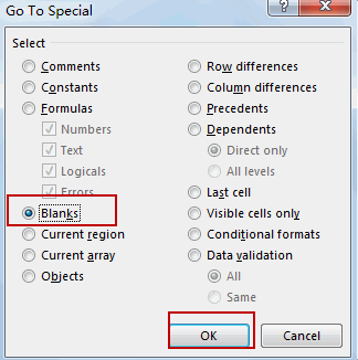
#4 click Blanks option in the Go To Special dialog. Click Ok button.

All of the blank cells have been selected in the selected range.

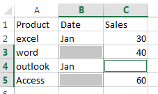
Note: You can click one of the following options to select all cells that contain specific types of data:

Click	To select
Comments	Cells that contain comments.
Constants	Cells that contain constants.
Formulas	Cells that contain formulas. Note: The check boxes below Formulas define the type of formula.
Blanks	Blank cells.
Current region	The current region, such as an entire list.
Current array	An entire array if the active cell is contained in an array.
Objects	Graphical objects, including charts and buttons, on the worksheet and in text boxes.
Row differences	All cells that differ from the active cell in a selected row. There is always one active cell in a selection—whether this is a range, row, or column. By pressing the Enter or Tab key, you can change the location of the active cell, which by default is the first cell in a row. If more than one row is selected, the comparison is done for each individual row of that selection, and the cell that is used in the comparison for each additional row is located in the same column as the active cell.
Column differences	All cells that differ from the active cell in a selected column. There is always one active cell in a selection, whether this is a range, row, or column. By pressing the Enter or Tab key, you can change the location of the active cell—which by default is the first cell in a column. When selecting more than one column, the comparison is done for each individual column of that selection. The cell that is used in the comparison for each additional column is located in the same row as the active cell.
Precedents	Cells that are referenced by the formula in the active cell. Under Dependents, do either of the following: Click Direct only to find only cells that are directly referenced by formulas. Click All levels to find all cells that are directly or indirectly referenced by the cells in the selection.
Dependents	Cells with formulas that refer to the active cell. Do either of the following: Click Direct only to find only cells with formulas that refer directly to the active cell. Click All levels to find all cells that directly or indirectly refer to the active cell.
Last cell	The last cell on the worksheet that contains data or formatting.
Visible cells only	Only cells that are visible in a range that crosses hidden rows or columns.
Conditional formats	Only cells that have conditional formats applied. Under Data validation, do either of the following: Click All to find all cells that have conditional formats applied. Click Same to find cells that have the same conditional formats as the currently selected cell.
Data validation	Only cells that have data validation rules applied. Do either of the following: Click All to find all cells that have data validation applied. Click Same to find cells that have the same data validation as the currently selected cell.

 

Find Cells That Meet one Criteria Using Conditional Formatting

---

You can also use the Conditional Formatting feature to find and select all cells that meet one certain criteria in your selected range.

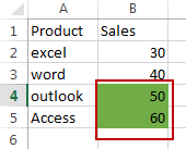
For example, you need to select cells that the sale values are greater than or equal to 50 in your selected range. Let’s do the following steps:

#1 select the range of cells that you want to use (B2:B5).

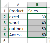
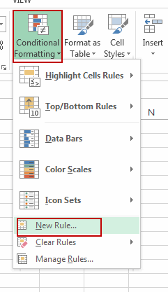
#2 go to HOME tab, click Conditional Formatting command under Styles group. And click New Rule from the drop down menu list. And the New Formatting Rule dialog will open.

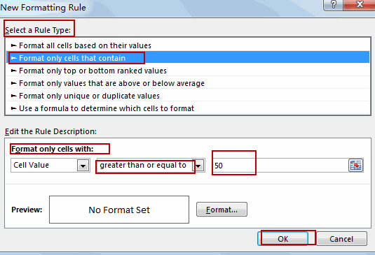
#3 select Format only cells that contain option under Select a Rule Type list box. Select greater than or equal to option from the second list box, and enter number 50 in the third box under Format only cells with section.

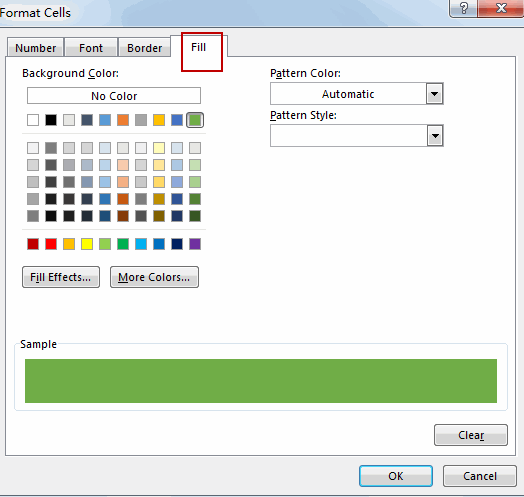
#4 Click Format button in the New Formatting Rule dialog, switch to Fill tab in the Format Cells dialog, and select one color as the background color. Click OK button.

#5 Click Ok button. The all of the Cells that are greater than or equal to number 50 have been find and highlighted with the color you set.