This post will guide you how to show milliseconds in Microsoft Excel. How do I format cells to time format to include milliseconds in Excel. In this post, you will learn different methods to show milliseconds in Excel, including using Format Cells Feature and Text function.

1. Show Milliseconds using Format Cells Feature

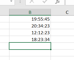
Assuming that you have a list of data in range B1:B4, in which contain time values, and if your time values contain milliseconds, when those time values are converted to time format, the milliseconds part will be disappeared. So if there is a way to keep to show milliseconds part in your time values. Just do the following steps:

Step 1: select the range of cells that contain time values.

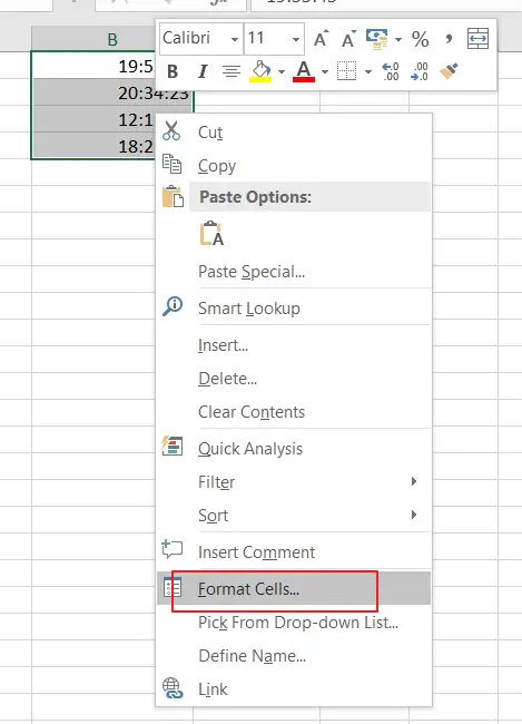
Step 2: right click on the selected cells, and select Format Cells from the context menu list. and the Format Cells dialog will open.

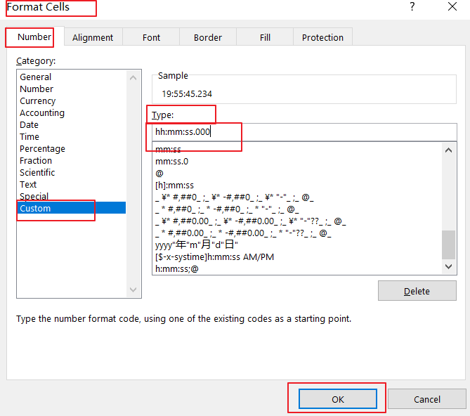
Step 3: switch to Number tab in the Format Cells dialog box, and click Custom in the Category list box, and type the format code hh:mm:ss.000 into the Type text box. and click Ok button.

Note: you need to include the “000” placeholder for milliseconds. The format code will dispaly timestamps with millisecond prescision, with three digits after the decimal point.If you need to adjust the format to match your specific timestamp data, you can modify the format code as needed.

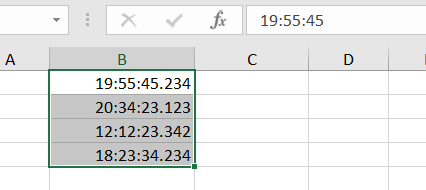
Step 4: you would see that the milliseconds are shown. And it will display the time in hours, minutes, seconds, and milliseconds.

2. Show Milliseconds by using Text Function

You can also use an Excel Formula based on the TEXT function to show milliseconds or add the milliseconds abbreviation or symbol to your time date.

Type the following formula in a black cell to display the time format in hours, minutes, seconds, and milliseconds:

=TEXT(B1,"hh:mm:ss.000")

If you want to add the milliseconds abbreviation on your time value, and you can use the “&” operator to concatenate the milliseconds values with the “ms” text, type the following formula:

=TEXT(B1,"hh:mm:ss") & "." & TEXT(B1,"000") & " ms"

3. How to Calculate the Average Time of a Set of Times with Milliseconds?

If you want to calculate the average time of a set of times given in hours, minutes, seconds and milliseconds in the selected range of cells in Excel, you can use the following formula based on the AVERAGE function, type:

=AVERAGE(B1:B4)*86400

The formula first calculates the average time in decimal format by using the AVERAGE function. It then multiplies the result by the number of seconds in a day (86400) to convert the decimal value back to the time format of minutes, seconds, and milliseconds.

Note: the above formula return a #DIV/0 error, and it may be the cells in the range B1:B4 are empty or contain non-numeric values.

If you want to exclude any non-numeric or empty cells in the given range to calculate the time values, and you can use the AVERAGEIF function, type”

=AVERAGEIF(B1:B4,">0")*86400

4. Conclusion

By following the simple steps outlined in this post, you can easily configure your Excel spreadsheets to show timestamps in milliseconds, which can be particularly helpful in your work.