If sum data by month in a table, we need to use a formula based on SUMIFS function. We can provide a set of conditions or criteria in SUMIFS function to sum data. To sum data by month, we need to add date range as criteria.
Table of Contents
Example:
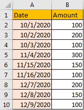
See below screenshot, if we want to sum total amount by month, how can we do?

Solution:
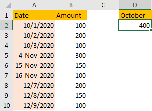
In C2, enter the formula =SUMIFS($B$2:$B$10,$A$2:$A$10,”>=”&A2,$A$2:$A$10,”<=”&EOMONTH(A2,0)).

Let’s see how this formula works:
For SUMIFS function, =SUMIFS(sum_range, criteria_range1, criteria1, [criteria_range2, criteria2], …), in this instance, $B$2:$B$10 is the sum range, $A$2:$A$10 is the criteria range, criteria 1 is >=A2 (10/1/2020), criteria 2 is <=EOMONTH(A2,0), it is the last date of October (the last date in month of A2), to get the last date in month of A2, we use EOMONTH function here.
For EOMONTH function, =EOMONTH(start_date, months), it returns the last date of a month for a specific date. In this instance, EOMONTH(A2,0), with zero as months value, it returns the last day of a month provided by date in A2. As A2 is 10/1/2020, so this function returns 10/31/2020 at last. In fact, it equals to =SUMIFS($B$2:$B$10,$A$2:$A$10,”>=10/1/2020″,$A$2:$A$10,”<=10/31/2020″). If you enter EOMONTH(A2,1), it will return the last date of next month based on date in A2, for example, A2 is 10/1/2020, then EOMONTH(A2,1) returns 11/30/2020. If you enter EOMONTH(A2,-2), it will return the last day of month, two months before the month in A2, in this case it is 8/31/2020.
Result:
Click Enter to get return value.

Notes:
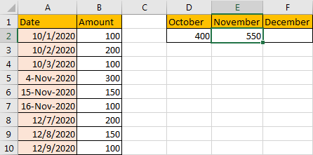
1. The formula also works if date format is other than mm/dd/yyyy. For example, we change date in November to different date format in table. Then formula is updated to =SUMIFS($B$2:$B$10,$A$2:$A$10,”>=”&A5,$A$2:$A$10,”<=”&EOMONTH(A5,0)).

It still works.

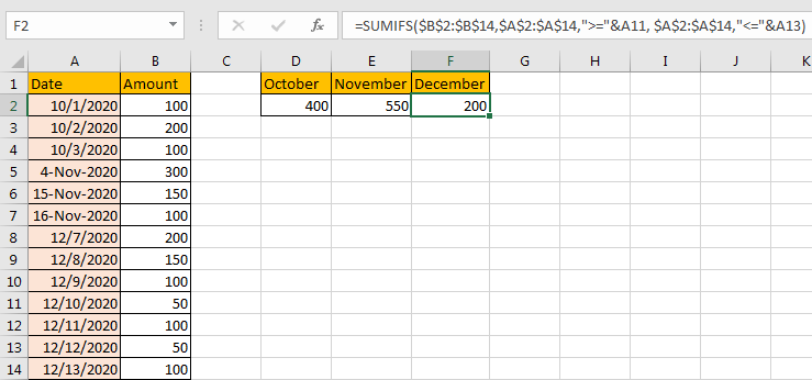
2. If we just want to sum data between a period, we can update formula to =SUMIFS(sum range, criteria range1,”>=”&start date, criteria range2,”<=”&end date). For example, to get amount between date 12/10/2020 and 12/12/2020. Enter the formula =SUMIFS($B$2:$B$14,$A$2:$A$14,”>=”&A11, $A$2:$A$14,”<=”&A13).

Related Functions
- Excel SUMIFS Function
The Excel SUMIFS function sum the numbers in the range of cells that meet a single or multiple criteria that you specify. The syntax of the SUMIFS function is as below:=SUMIFS (sum_range, criteria_range1, criteria1, [criteria_range2, criteria2], …)…