To generate a business summary report for further investigation, we can sum income or profits for a date like Monday, Tuesday …etc. to check on which date we have the top income in a week, then we can estimate the market trend. Actually, sum data by weekday is a common operation in our daily life, when generating report, we often select one or more weekdays as a period to sum data. So, it is necessary for us to have the knowledge of sum data by weekday in excel. Actually, excel built-in functions SUMIFS and SUMPRODUCT can help us resolve this issue properly.
This article will show you ‘Sum by Weekday’ in two different ways via excel WEEKDAY, SUMIFS and SUMPRODUCT functions with simple examples, descriptions, screenshots and explanations, and we will let you know how these formulas work with these functions. Besides, there are some differences in the usage of the two functions SUMIFS and SUMPRODUCT even though they are both used for sum data. Read the following article, you can learn sum data by formula clearly by yourself, you can select one way you feel easy to understand to achieve your goal, and you can work well with these functions in your daily work in the future.
EXAMPLE:
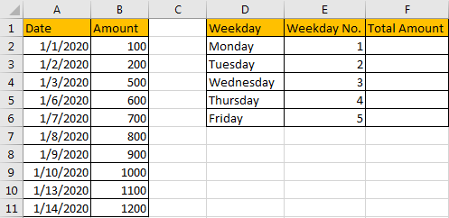
Table of Contents
METHOD 1: APPLY SUMIFS FUNCTION TO SUM DATA BY WEEKDAY
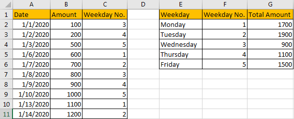
As we can see that there is a column in the right table called ‘Weekday No.’, actually each value reflects a weekday accordingly, for example 1 reflects Monday, 2 reflects Tuesday… and 5 reflects Friday. So, we can also create a helper column called ‘Weekday No.’ in the left table, then we can use SUMIFS function contains ‘Weekday No.’ as criteria range to sum data by weekday properly. Refer to this method, the first step we need to get weekday numbers for all entered data in ‘Date’ list. So, create a helper column, enter the formula =WEEKDAY(A2,2) in the blank cell, see screenshot below.
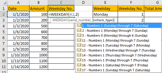
As generally if you omit ‘return type’ in WEEKDAY function, Sunday will be assigned with weekday number 1 by default, so the weekday numbers are inconsistent in two ‘Weekday No.’ columns. So here we enter ‘2’ as return type, then Monday will be assigned with weekday number 1.
After clicking Enter, the formula returns ‘3’ as result. That means date 1/1/2020 is Wednesday.

Drag down the cell to copy the formula. Then we can get all weekday numbers for entered dates.
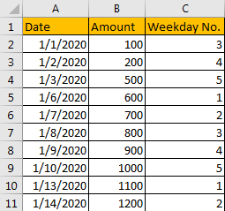
Now, Weekday No. in C column can be seen a criteria range for SUMIFS function, and each number in ‘Weekday No.’ in F column can be seen as criteria of it. Now, we can apply SUMIFS function in this instance to sum data per weekday.
In G1 enter the formula =SUMIFS($B$2:$B$11,$C$2:$C$11,F2). After clicking Enter, we can get correct total amount 1700, that means the formula works correctly.
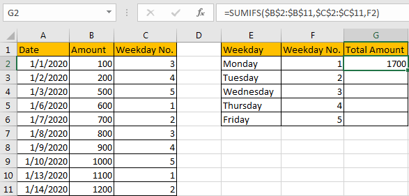
HOW THIS FORMULA WORKS:
This formula contains two functions, we explain the formula from inside to outside. Firstly, we apply WEEKDAY function in this instance. WEEKDAY function can return the day of a week, it returns an integer, and the integer range is 1 to 7, normally 1 represents Sunday, 2 represents Monday etc., and 7 represents Saturday. The syntax is consistent of WEEKDAY(serial_number,[return_type]).
You can enter a date within double quote in the function. For example, enter =WEEKDAY(“10/22/2020”), click Enter, we will get 5. That means 10/22/2020 is Thursday.

But if you want to set 1 to represent Monday, 2 represent Tuesday and 7 represent Sunday respectively, we can add return type 2 into WEEKDAY function. Now 4 is returned as we expect.

We can also select a cell number directly when applying this function. In this instance, we can get correct weekday number after applying the formula.

Then we apply SUMIFS function =SUMIFS($B$2:$B$11,$C$2:$C$11,F2) to sum data. For SUMIFS function, it sums data with multiple criteria, the syntax has some arguments, see below:
=SUMIFS(sum_range, criteria_range1, criteria1, [criteria_range2, criteria2], …).
$B$2:$B$11 is the sum range, it provides values to sum, as it is an absolute range in this case, so we add $ before row and column number to lock the range, so when copying formula to other cells, this range is fixed, user doesn’t need to adjust the sum range any more.
$C$2:$C$11 is the criteria range, it provides all weekday numbers, it is an absolute range in this case as well, so we add $ before row and column number.
F2 is the criteria of criteria range $C$2:$C$11.
We compare each value in criteria range $C$2:$C$11 with the value in F2, if they are consistent, corresponding amount value in sum range $B$2:$B$11 will be accumulated. By this way, we get total amount for each weekday.
RESULT:
Let’s check if the formula works well for other weekdays.
METHOD 2: APPLY SUMPRODUCT FUNCTION TO SUM DATA BY WEEKDAY
The above instance uses a helper column ‘Weekday no.’ to sum data, without helper column SUMIFS function cannot work due to there is no criteria. If we want to sum data by weekday without helper column and just use the given data in tables, how can we do?
Actually, we can through applying another excel function to achieve our requirement.
FORMULA:
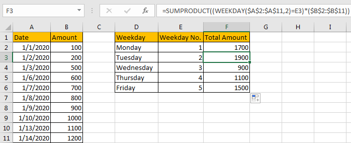
In F1 enter the formula =SUMPRODUCT((WEEKDAY($A$2:$A$11,2)=E2)*($B$2:$B$11)).

Click Enter to check returned value.

Verify that total amount is 1700, it is consistent with the value summed by SUMIFS function in former instance.
HOW THIS FORMULA WORKS:
Unlike SUMIFS function, SUMPRODUCT function syntax has the following arguments:
=SUMPRODUCT(array1, [array2], [array3], …)
In this instance, in the formula SUMPRODUCT((WEEKDAY($A$2:$A$11,2)=E2)*($B$2:$B$11)), there is only one argument (WEEKDAY($A$2:$A$11,2)=E2)*($B$2:$B$11). In method #1, we have explained the usage of WEEKDAY, here, as we enter $A$2:$A$11 as serial number, so WEEKDAY($A$2:$A$11,2) will return an array instead of an integer; as return type is ‘2’, so if date is Monday, 1 is returned in array.
In this instance, WEEKDAY($A$2:$A$11,2) returns the array {3;4;5;1;2;3;4;5;1;2}.

(Select WEEKDAY($A$2:$A$11,2) in formula bar, and press F9, then returned array will be displayed.)
Just pick up each value from the array list, and compare it with the value in E2 (1 in this case). {3;4;5;1;2;3;4;5;1;2}=1.

After comparing, we can get the result as below:
{FALSE;FALSE;FALSE;TRUE;FALSE;FALSE;FALSE;FALSE;TRUE;FALSE}

As function cannot work with TRUE or FALSE, so they are forced to be converted to numbers. Convert FALSE to 0 and TRUE to 1 for following work. So, the array is updated to {0;0;0;1;0;0;0;0;1;0}.
$B$2:$B$11 is the sum range {100;200;500;600;700;800;900;1000;1100;1200}.

So, SUMPRODUCT((WEEKDAY($A$2:$A$11,2)=E2)*($B$2:$B$11)) can be seen as one array is multiplied by the values in another array:
{0;0;0;1;0;0;0;0;1;0}*{100;200;500;600;700;800;900;1000;1100;1200}={0;0;0;600;0;0;0;0;1100;0}. Then sum the values in the array, the final result is 1700, see screenshot below.

RESULT:
Let’s see if this formula works correctly for other weekdays. Obviously, it works well.
NOTES:
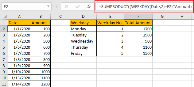
If you are confused of range selection in the formula, you can also name range firstly, for example
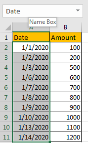
$A$2:$A$11=Date;
$B$2:$B$11=Amount;
To name range, just select the whole range (for example A2:A11, ignore the header), and enter name in name box (for example ‘Date’). Please be aware that there should be NO space in range name.
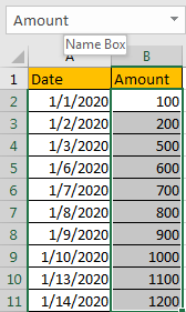
Then update formula to =SUMPRODUCT((WEEKDAY(Date,2)=E2)*Amount). It looks clearly now.
Related Functions
- Excel SUMPRODUCT function
The Excel SUMPRODUCT function multiplies corresponding components in the given one or more arrays or ranges, and returns the sum of those products.The syntax of the SUMPRODUCT function is as below:= SUMPRODUCT (array1,[array2],…)… - Excel WEEKDAY function
The Excel WEEKDAY function returns a integer value representing the day fo the week for a given Excel date and the value is range from 1 to 7.The syntax of the WEEKDAY function is as below:=WEEKDAY (serial_number,[return_type])… - Excel SUMIFS Function
The Excel SUMIFS function sum the numbers in the range of cells that meet a single or multiple criteria that you specify. The syntax of the SUMIFS function is as below:=SUMIFS (sum_range, criteria_range1, criteria1, [criteria_range2, criteria2], …)…