We often sum data based on criteria. To sum values based on a cell, in fact, we sum values based on the text in this cell. If the text is included in another table another column, we need to find out all locations of this text in this column, and then sum up all matched values to the column.

In this article, we will show you the formula which can ‘sum if cell contains text in another column’ with the application of SUMIFS function. Through a simple instance, we will introduce you the syntax, arguments of SUMIFS function, and let you know how each part within the formula works for getting the correct result we expect. After reading the article, you can have a simple understanding of SUMIFS function, and you may use it properly in more cases.

1. Sum if Cell Contains Text in Another Column using Formula

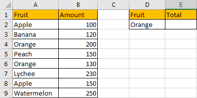
In the left table, we list different kinds of fruits in column A, some are duplicate. We list amounts for these kinds of fruits in column B.

In the right table, we enter one kind of fruit in cell D2, it is included in column A fruit list. It is a dynamic value, we can enter any kind of fruit into this field, just make sure that the entered fruit always exists in column A. Then, though entering a formula in ‘Total’ E2, we can get proper total amount dynamically based on the entered fruit in D2.

Above all, to edit this formula, we will apply Excel SUMIFS function.

FORMULA – SUMIFS FUNCTION

Step 1: In E2, enter the formula =SUMIFS(B2:B9,A2:A9,D2).

Step 2: Press Enter after typing the formula.

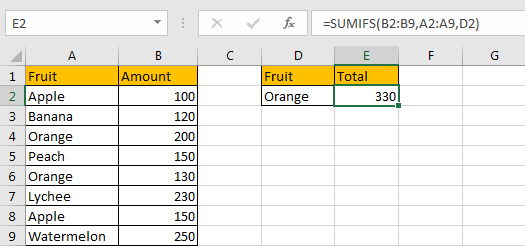
We can see in column A there are two cells contain text ‘Orange’, the corresponding amounts are 200 and 130, so the total is 200+130=330. It can be seen the formula works correctly.

SUMIFS FUNCTION INTRODUCTION

SUMIFS function can be seen as SUM+IFS, it supports multiple ‘criteria range’ and ‘criteria’ combinations.

For SUMIFS function, the syntax is:

SUMIFS(sum_range, criteria_range1, criteria1, [criteria_range2, criteria2], …).

Criteria range N and criteria N are optional, so it still works if only one criteria range and one criterion exist.

To let you know the application of SUMIFS function in our formula in this instance, we will explain each argument in SUMIFS function, and split the formula to several parts, let you know how it works from inside to outside.

ALL ARGUMENTS

SUMIFS – SUM RANGE

In our instance, B2:B9 is the sum range, it provides values to sum up. If we want to set it as an absolute range, we can add $ before column and row to lock the range, like this $B$2:$B$9. Then when copying formula to other cells, this range is fixed.

Actually, in range B2:B9, each cell saves a value, if we save these values in an array, it is:

{100;120;200;150;130;230;150;250}

In formula bar, select B2:B9, press F9, values in this range are listed in an array.

SUMIFS – CRITERIA RANGE

A2:A9 is the criteria range, in this case we have only one criteria range. Similar with B2:B9, it records all fruits, some of them are duplicate, if we list them in an array, it looks like:

{“Apple”;”Banana”;”Orange”;”Peach”;”Orange”;”Lychee”;”Apple”;”Watermelon”}

In the formula bar, it displays:

SUMIFS – CRITERIA

In this formula, D2 is the criteria, it contains text ‘Orange’.

HOW FORMULA WORKS

After introducing each argument, we get two arrays and a text, see the formula below:

=SUMIFS({100;120;200;150;130;230;150;250},{“Apple”;”Banana”;”Orange”;”Peach”;”Orange”;”Lychee”;”Apple”;

“Watermelon”},”Orange”)

In the formula, the criteria range and criteria are:

Criteria range: {“Apple”;”Banana”;”Orange”;”Peach”;”Orange”;”Lychee”;”Apple”;”Watermelon”}

Criteria: “Orange”

In the range, “Orange” occurs twice; compare each value in array with text “Orange”, only the two fields are True, others are False.

So, after comparing with criteria range with criteria, we get below array:

{False;False;True;False;True;Flase;False;False}

Convert ‘True’ to ‘1’ and ‘False’ to ‘0’:

{0;0;1;0;1;0;0;0}

Now, we have below two arrays:

Array 1: {100;120;200;150;130;230;150;250} – sum range

Array 2: {0;0;1;0;1;0;0;0} – criteria

The two arrays are matched. So, in array1, value will be saved only if its corresponding value in array2 is “1”, otherwise, “0” will be recorded in current array instead of the original value.

Refer to above rule, we get an updated array1:

Array 1: {0;0;200;0;130;0;0;0} – updated sum range

Now, sum up existing values in array1.

0+0+200+0+130+0+0+0=330

After all, we get the result 330.

COMMENTS

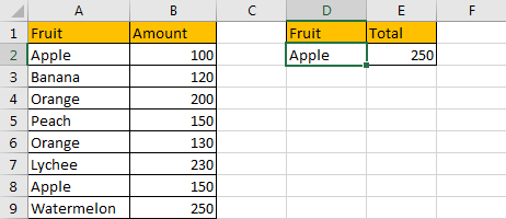
1. We can enter another fruit into D2, the total value is updated accordingly.

2. In this formula, instead of enter cell reference ‘D2’, we can enter ‘Orange’ into formula directly.

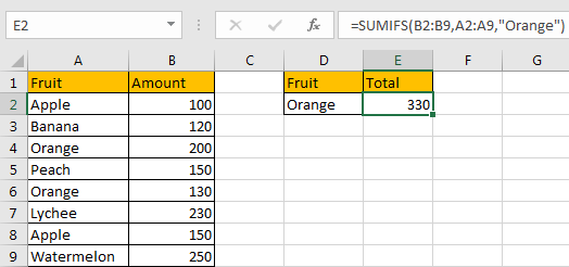
Be aware that you have to add double quotes “” and make sure the text is within “”.

If you forgot “”, then “0” is returned.

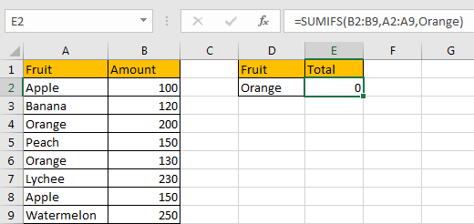
3. If in column A, cell contains text “Orange”, but not equals to “Orange”, the formula cannot work properly. See example below:

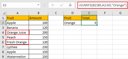
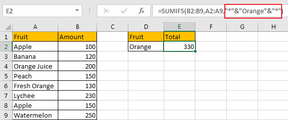
In this case, we need to add “*” before and after “Orange”.

Or add “*” before and after D2 (without double quotes).

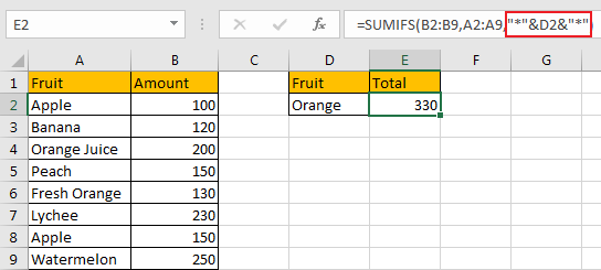
Actually, SUMIFS function can support wildcards in its formula, and it requires to add double quotes (““) to enclose wildcards or texts.

1. An asterisk (*) means one or more characters.
2. A question mark (?) means one character.
3. The position of asterisk or question mark means the character(s) position relative to the entered part.

4. You can define sum range and criteria range with proper names, then enter defined names into formula respectively.

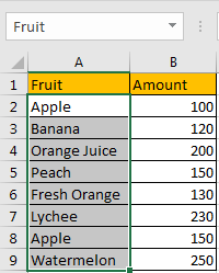
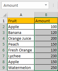
For example, select range A2:A9, in ‘Name Box’ enter ‘Fruit’ to name this range; select B2:B9, name this range ‘Amount’.

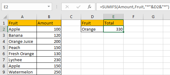
So enter =SUMIFS(Amount,Fruit,”*”&D2&”*”) instead of former formula, we still get proper result.

2. Sum if Cell Contains Text in Another Column using VBA Code

Let’s see the second method, we’ll leverage the power of VBA to automate the process of summing values based on certain conditions. With VBA code, we can create custom functions to efficiently handle complex tasks in Excel.

Press ‘Alt + F11‘ to open the Visual Basic for Applications (VBA) editor.

Right-click on any item in the project explorer (on the left), hover over “Insert,” and select “Module” to add a new module.

In the newly created module, copy and paste the following VBA code:

Function SumIfContainsText(criteriaRange As Range, sumRange As Range, criteria As String) As Double
    Dim cell As Range
    Dim sumValue As Double
    
    For Each cell In criteriaRange
        If cell.Value = criteria Then
            sumValue = sumValue + sumRange.Cells(cell.Row - criteriaRange.Row + 1).Value
        End If
    Next cell
    
    SumIfContainsText = sumValue
End Function

Close the VBA editor by clicking the “X” button or pressing ‘Alt + Q.’

Return to your Excel workbook.

In a blank cell, enter the formula like this:

=SumIfContainsText(A2:A9, B2:B9, D2)

Replace “A2:A9” with the range containing the text criteria, “B2:B9” with the range containing the values to be summed, and “D2” with the specific text to match.

Press Enter to execute the formula and obtain the sum.

The VBA function will sum values based on the text criteria provided in another column.

3. Video: Sum if Cell Contains Text in Another Column

This Excel video tutorial on how to sum if a cell contains text in another column. In this video, we’ll explore two methods: using formulas and VBA code to achieve this task efficiently.