In previous article, we have introduced you the method to sum if by year, you can check “How to Sum Data if by Year in Excel” on our website for reference. But sometimes we may want to sum numbers not for a year but just for a period. In this article, we will show you how to ‘sum if date between two dates’ by formula with the help of Excel SUMIFS function. Due to date format issue may occurs in real life, we also introduce DATE function in case of you meet the same problem as we describe in example2.

Through a simple instance, we will introduce you the syntax, arguments of SUMIFS function, and let you know how the formula works step by step to reach your goal finally. After reading the article, you may have a simple understanding of SUMIFS function.

EXAMPLE

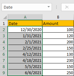
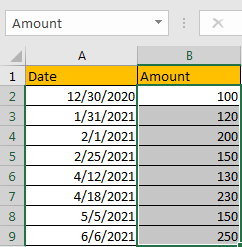
Refer to above left-hand table, we can see that in the most left column “Date”, some dates are listed. And amount for each date is listed in “Amount” column accordingly.

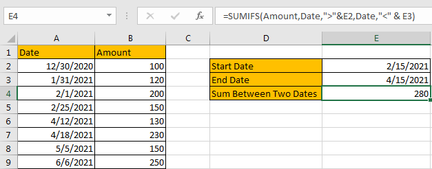
In this instance, we want to sum numbers between a period. And this period is confirmed by the two dates “Start Date” and “End Date” in the right-hand table. This period is a dynamic period due to we can change “Start Date” and “End Date” based on our requirement. After the period is provided, only the dates which are between this period can meet our condition. We need to find out all proper dates, and then sum up values in “Amount” column. To resolve this issue by formula, we can apply SUMIFS functions.

FORMULA – SUMIFS FUNCTION

Step 1: Select A2:A9, then in Name Box define a new name for this range, for example ‘Date’.

Step 2: Select B2:B9, in Name Box define a new name for this range, for example ‘Amount’.

Step 3: In E4, enter the formula =SUMIFS(Amount,Date,”>”&E2,Date,”<” & E3).

NOTE: In step#1 and step#2 we defined range name “Date” and “Amount”, when entering the formula, after typing “Amou…”, defined range “Amount” is auto loaded, you can directly select it from dropdown list. You can also select B2:B9, A2:A9 to fill formula arguments as well.

Step 4: Press Enter after typing the formula.

We can see in column A, cell A5 (2/25/2021) and A6 (4/12/2021) just between period “2/25/2021-4/15/2021”, the corresponding amounts are 150 (in cell B5), 130 (in cell B6), and 150 (in cell B8), so the total amount is 150+130=280. The formula works correctly.

SUMIFS FUNCTION INTRODUCTION

SUMIFS function can be seen as SUM+IFS, it can handle multiple ‘criteria range’ and ‘criteria’ combinations.

For SUMIFS function, the syntax is:

SUMIFS(sum_range, criteria_range1, criteria1, [criteria_range2, criteria2], …). Contents in [] are optional.

SUMIFS function supports wildcards like asterisk ‘*’ and question mark ‘?’, it also supports logical operators within its arguments. If wildcards or logical operators are required, they should be enclosed into double quotes (““) with text.

The usage of wildcards:

1. An asterisk (*) means one or more characters.
2. A question mark (?) means one character.
3. The position of asterisk or question mark means the character(s) position relative to the entered part. For example, “*A*” means characters or texts are both listed before and after “A”. “A*” means this text is started with A, but ends with others.

The usage of logical operators:

1. “>” – greater than
2. “>=” – greater than or equal to
3. “<” – less than
4. “<” – less than or equal to
5. “<>” – not equal to

ALL ARGUMENTS

SUMIFS – SUM RANGE

In our instance, B2:B9 is the ‘sum range’ obviously. Amount values are listed in this field. We define this range with name ‘Amount’ in above step#2.

In the formula bar, select ‘Amount’, press F9, values in this range are listed in an array.

SUMIFS – CRITERIA RANGE 1

A2:A9 is the criteria range. In this instance we have only one criteria range. This range contains different dates.

In the formula bar, select ‘Date’, press F9, values in this range are listed in an array.

In this step, dates are converted from Date format to General format, a five digits number is displayed to represent a date. Date 12/30/2020 in A2 is the earliest date in the list, so its relative five digits number 44195 is the smallest in the array, and date 6/6/2021 is the latest date in the list, so 44353 is the largest among all numbers in the array.

SUMIFS – CRITERIA 1

We want to calculate total amount for the period between start date “2/15/2021” and end date “4/15/2021”. The two dates are saved in E2 and E3, we can directly enter cell reference in the formula to stand for the two dates. As the target date should be included in the two dates, that means it is greater than the start date (>E2) and at the mean time it is also smaller than the end date (<E3).

Thus, the first criteria should be “greater than the date in E2”. As we explained above, SUMIFS function allows logical operators, but they should be enclosed into double quotes “”, so for criteria 1, we enter logical operator > within quotes as “>”. And to concentrate logical operator and cell reference E2, we add & between them. Please be aware that if you enter “>”E2 without & into formula, formula cannot accept this combination and directly quit entering. After all, for criteria 1, we enter “>”&E2.

E2=2/15/2021, convert it to general format in the formula bar, it is 44242.

SUMIFS – CRITERIA RANGE 2

It is still range A2:A9.

SUMIFS – CRITERIA 2

The second criteria should be “smaller than the date in E3”. So we enter “<”&E3 in the formula.

E3=4/15/2021, convert it to general format in the formula bar, it is 44301.

HOW FORMULA WORKS

After explaining each argument in the formula, now we will show you how the formula works with these arguments.

Refer to above mentioned arguments, the formula is converted into below format in the formula bar.

=SUMIFS({100;120;200;150;130;230;150;250},{44195;44227;44228;44252;44298;44304;44321;44353},”>”&44242,{44195;44227;44228;44252;44298;44304;44321;44353},”<“&44301)

See screenshot below:

See the two pairs of criteria range and criteria:

Criteria range 1: {44195;44227;44228;44252;44298;44304;44321;44353}

Criteria 1: “>”&44242

In criteria range 1, compare each number in the array with criteria 44242; if number can satisfy the condition “>44242”, mark it bold in array:

{44195;44227;44228;44252;44298;44304;44321;44353} – Bold if it is >44242

Criteria range 2: {44195;44227;44228;44252;44298;44304;44321;44353}

Criteria 2: “<“&44301

In criteria range 2, compare each number in the array with criteria 44301; if number can satisfy the condition “<44301”, mark it bold in array:

{44195;44227;44228;44252;44298;44304;44321;44353} – Bold if it is <44301

Find out the intersection between two arrays. The result can meet our requirement “between 44242 and 44301” which means “between the period 2/15/2021 and 4/15/2021”.

{44195;44227;44228;44252;44298;44304;44321;44353} – Bold if it is just between 44242 and 44301.

Now, for bold numbers, they can meet our requirement, so record a ‘True’ for them in the array; otherwise, record a ‘False’ for others. Then we can get a new array:

{Flase;False;False;True;True;False;False;False}

Convert ‘True’ to ‘1’ and ‘False’ to ‘0’ to apply this array into calculation in the following steps:

{0;0;0;1;1;0;0;0}

Now, we have below two arrays:

{100;120;200;150;130;230;150;250} – Sum Range

{0;0;0;1;1;0;0;0} – from above steps we know that if date is included in the period, 1 is displayed.

We list the two arrays in two rows, in the same column multiply the two numbers, and save their product in another row.

Sum up all numbers in the third row.

150+130=280

EXAMPLE 2

Sometimes dates are not just displayed in proper date format which can be directly applied in formula as we expect. They can be displayed in some other date formats in worksheet, see example below:

In this situation, if you want to sum numbers based on period, you should hard code dates by DATE function, then refer to above method to apply SUMIFS function.

FORMULA – SUMIFS AND DATE FUNCTIONS

Step 1: In E4, enter the formula =SUMIFS(Amount,Date,”>”&DATE(2021,2,15),Date,”<“&DATE(2021,4,15)).

Step 2: Press Enter after typing the formula.

DATE FUNCTION INTRODUCTION

DATE function can return a serial number that can represent a particular date if current cell format is ‘General’ or directly return a date if current cell format is ‘Date’. The syntax is

DATE(year,month,day) – All the three arguments ‘year’,’month’,’day’ are required.

HOW FORMULA WORKS

 

We applied DATE function twice in this case, the start date is 15-Feb-2021, end date is 15-Apr-2021, so in the first DATE function we enter DATE(2021,2,15), and the second DATE function we enter DATE(2021,4,15).

In the formula bar, select “DATE(2021,2,15)”, press F9, date is converted to a five digits number 44242.

Then select “DATE(2021,2,15)”, press F9, date is converted to a five digits number 44301.

Now, we get the two numbers, the following steps are as same as example1.

SUMMARY

1. SUMIFS function can handle multiple groups of criteria ranges and criteria. Sum range is the first argument among all arguments.

2. It supports user defined range name.

3. It supports wildcard.

4. It supports logical operators.

If you want to hard-code date in formula, you can apply DATE function.

Related Functions

---

• Excel SUMIFS Function
  The Excel SUMIFS function sum the numbers in the range of cells that meet a single or multiple criteria that you specify. The syntax of the SUMIFS function is as below:=SUMIFS (sum_range, criteria_range1, criteria1, [criteria_range2, criteria2], …)…
• Excel DATE function
  The Excel DATE function returns the serial number for a date.The syntax of the DATE function is as below:= DATE (year, month, day)…