We may meet the case that sum numbers based on a certain value in daily work. To sum numbers based on a certain value, we can define this value as a criterion. Then sum up all numbers which meet the condition. The scenario can be simple or complex in real life. But no matter how complex it is, we can use proper excel function to resolve problem.
In this article, we will show you the resolution of ‘sum if cells equal to a certain value’ by formula with the help of Excel SUMIFS function. Through demonstrate a simple instance, we will introduce you the syntax, arguments of SUMIFS function, and let you know how this formula works for reaching the target. Actually, some other functions like SUMIF (or the combination of excel functions) can also resolve this issue, we will also mention SUMIF function a little bit in the end to let you know another way of sum number with condition. After reading the article, you may have a simple understanding of SUMIFS function, and also a supplement of you excel skills
EXAMPLE
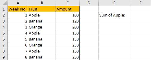
Refer to above table, we can see that we sale only one kind of fruit each week. We list week number in column A, some kinds of fruits in column B, fruits are on sale alternatively. Total amount for each week for specific fruit is listed in column C.
In this instance, we want to calculate total amount for apple. That means we need to sum up data in column C which B column in the same row equals to ‘Apple’ exactly. We can apply a formula contains SUMIFS function to resolve this issue.
FORMULA – SUMIFS FUNCTION
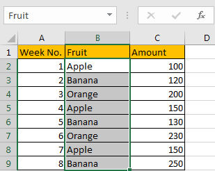
Step 1: Select B2:B9, then in Name Box define a new name for this range, for example ‘Fruit’.
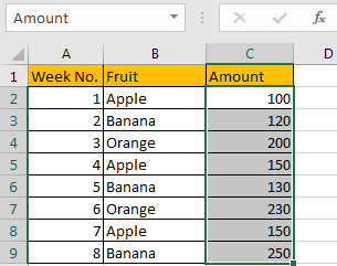
Step 2: Select C2:C9, in Name Box define a new name for this range, for example ‘Amount’.
Step 3: In F2, enter the formula =SUMIFS(Amount,Fruit,”Apple”).

Step 4: Press Enter after typing the formula.
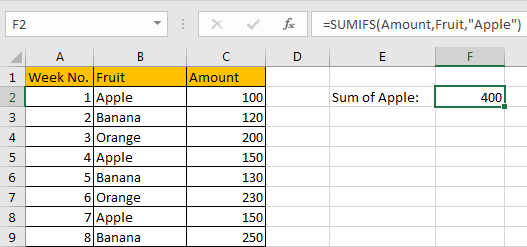
We can see in column A there are three cells are equal to text ‘Apple’, the corresponding amounts are 100 (in cell C2), 150 (in cell C5) and 150 (in cell C8), so the total is 100+150+150=400. The formula works correctly.
SUMIFS FUNCTION INTRODUCTION
SUMIFS function can be seen as SUM+IFS, it can handle multiple ‘criteria range’ and ‘criteria’ combinations.
For SUMIFS function, the syntax is:
SUMIFS(sum_range, criteria_range1, criteria1, [criteria_range2, criteria2], …). Contents in [] are optional.
ALL ARGUMENTS
SUMIFS – SUM RANGE
In our instance, C2:C9 is the sum range obviously. We define this range with name ‘Amount’ in precondition, it is easy to understand than just entering ‘C2:C9’ in sum range position in formula.
In the formula bar, select ‘Amount’, press F9, values in this range are listed in an array.

SUMIFS – CRITERIA RANGE
B2:B9 is the criteria range. In this instance we have only one criteria range. This range contains three kinds of fruits.
In the formula bar, these fruits are displayed in proper order in an array:

SUMIFS – CRITERIA
We want to calculate total amount for ‘Apple’ only. We need to look up all cells equal to ‘Apple’ from criteria range. So, in criteria position we enter ‘Apple’. SUMIFS function supports texts, but they should be enclosed into double quotes “ “ when applying them.

HOW FORMULA WORKS
After introducing each argument, we get two arrays and a text within double quotes, the formula is converted into below format in the formula bar.
=SUMIFS({100;120;200;150;130;230;150;250},{"Apple";"Banana";"Orange";"Apple";"Banana";"Orange";"Apple";"Banana"},"Apple")
See screenshot below:
![]()
As mentioned above, the criteria range, criteria are:
Criteria range: {“Apple”;”Banana”;”Orange”;”Apple”;”Banana”;”Orange”;”Apple”;”Banana”}
Criteria: “Apple”
In criteria range, “Apple” occurs three times, at the first position, the fourth position and the seventh position; So, these positions are marked with ‘True’ after comparing with text ‘Apple’, the others are not ‘Apple’, so they are marked with ‘False’.
So, after comparing we get below array:
{True;False;False;True;False;Flase;True;False}
Convert ‘True’ to ‘1’ and ‘False’ to ‘0’:
{0;0;1;0;1;0;0;0}
Now, we have below two arrays:
Array 1: {100;120;200;150;130;230;150;250} – sum range
Array 2: {1;0;0;1;0;0;1;0} – if cell equals to ‘Apple’, 1 is displayed.
We list the two arrays in two rows, and create a new array ‘Array3’ to save numbers based on different values in array2. For example, in array1, value will be copied to array3 only if array2 value in the same column is “1”, otherwise, “0” will be recorded in array3 instead of the original value. So, we get below table finally:

In array2, 1 means in this position the original value is ‘Apple’; Array1 records amount for each kind of fruit in array2. Above all, numbers which are not zero in array3 are the amounts of ‘Apple’ after filtering. Now, sum up all values in array3.
100+0+0+150+0+0+150+0=400
Above analysis can help us know the process of this formula reaching the goal step by step clearly.
COMMENTS
1. To understand the formula easily, we define range name in precondition. If you ignore this step, you can directly enter the range reference in formula.
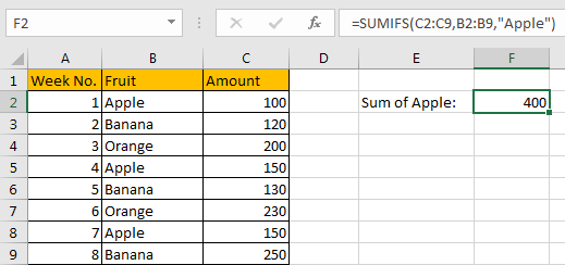
2. For this instance, you can also apply SUMIF function.
Enter =SUMIF(B2:B9,”Apple”,C2:C9) instead of applying SUMIFS formula.
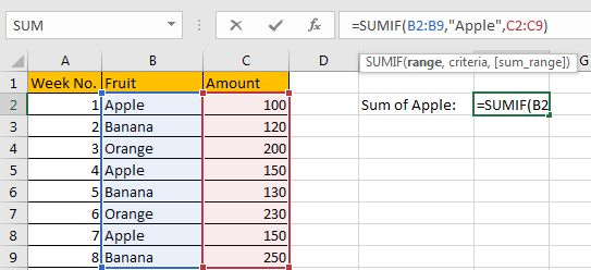
We can get the same result. You can see that the order of arguments is a little different than SUMIFS function.
SUMMARY
1. SUMIFS function can handle multiple groups of criteria ranges and criteria. Sum range is first argument among all arguments.
2. SUMIFS function supports user defined range name.
Related Functions
- Excel SUMIF Function
The Excel SUMIF function sum the numbers in the range of cells that meet a single criteria that you specify. The syntax of the SUMIF function is as below:=SUMIF (range, criteria, [sum_range])… - Excel SUMIFS Function
The Excel SUMIFS function sum the numbers in the range of cells that meet a single or multiple criteria that you specify. The syntax of the SUMIFS function is as below:=SUMIFS (sum_range, criteria_range1, criteria1, [criteria_range2, criteria2], …)…