Suppose we have two lists in excel, one list records the product serial numbers, these serial numbers can be duplicate, and the other list records the sales volume for products accordingly, for more details you can see the screenshot in precondition below. To calculate the total sales volume, normally we can use SUM function in excel. But if we only want to sum the sales volume for only one product, how can we do? In a traditional way, we can do filter firstly to filter out the product we want, then calculate the total values one by one. But this way is boring and time-consuming especially the data amount is large. Above all, we need to find another simple way to sum values for specified product to meet our requirement. This free tutorial will introduce you a convenient way to sum total values based on criteria, you cannot miss it.
Precondition:
See screenshot below, we prepare two lists, the first column records the product serial number, the second one records the income for all products. We can see that some products are duplicate in the list, if we want to calculate the total income for these products, in a traditional way we have to sum all of them one by one.
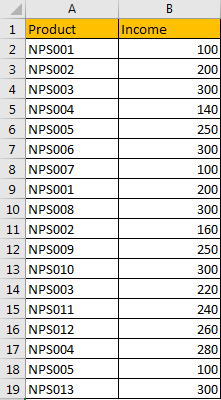
Table of Contents
1. Sum Values Based on Criteria in Another Column
Step 1: Copy ‘Product’ column to another column first.
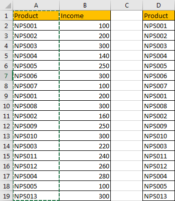
Step 2: On column D, click Data in ribbon, then click Remove Duplicate under Data Tools group.

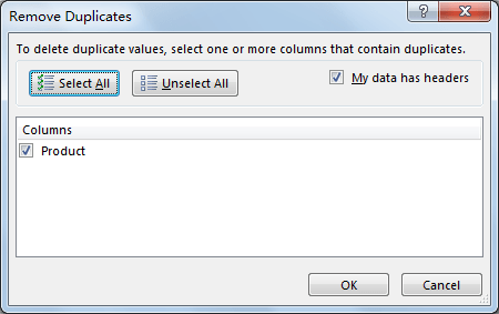
Step 3: ‘Remove Duplicates’ dialog pops up. Just click OK.
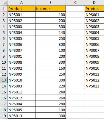
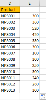
The you will notice that duplicate values are removed from column D. All products are unique.
Step 4: Select a blank cell next to the filtered product list, for example E2, enter the following formula:
=SUMIF($A$2:$A$19, D2, $B$2:$B$19).
Step 5: Click Enter to get result. Verify that total income is calculated properly.

Step 6: Drag the fill handle down till the end of list. Verify that total income is calculated properly for each product.
2. Sum Values Based on Criteria by PivotTable
We can also calculate total income for all products via excel PivotTable.
Step 1: Select the range A1:B19, then click Insert in ribbon, click PivotTable to create a PivotTable for the selected range.

Step 2: After above operating, ‘Create PivotTable’ dialog pops up. Choose the location to save PivotTable. We choose existing workbook and started cell G1 to save it. Then click OK.

Step 3: On PivotTable Fields screen, check on Product and Income, move Product under Rows, under Values select ‘Sum of Income’.
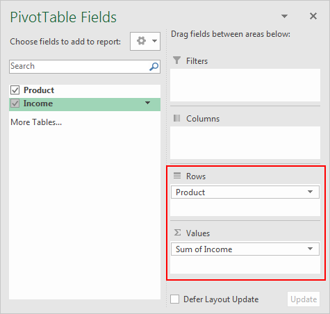
Step 4: Verify that PivotTable for the selected range is inserted properly.
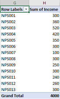
You can select the small arrow button to select product to see the sum of income.

3. Video: Sum Values Based on Criteria
This Excel video tutorial, where we’ll unravel the method of summing values based on a criteria list in another column. In this session, we’ll explore two efficient methods – the formula-based approach using the SUMIF function and the power-packed PivotTable.
4. Related Functions
- Excel SUMIF Function
The Excel SUMIF function sum the numbers in the range of cells that meet a single criteria that you specify. The syntax of the SUMIF function is as below:=SUMIF (range, criteria, [sum_range])… - Excel SUM function
The Excel SUM function will adds all numbers in a range of cells and returns the sum of these values. You can add individual values, cell references or ranges in excel.The syntax of the SUM function is as below:= SUM(number1,[number2],…)…