We can do SUM for a list or a range of values easily if we select all values together and then apply SUM function in excel. But if we only want to sum part of them based on the selection in a dropdown list, how can we do? For example, suppose we have two lists, one list records some fruits, and they can be duplicate in this list, the other list records the amount, if we create a filter on fruits and just pick one of them, how can we sum the total amount of this filtered fruit. Though we can calculate the total amount one cell by another cell, this is not very simple. So, in this free tutorial, we will introduce you a simple way (through a formula) to sum values based on the selection of dropdown list.
Precondition:
Prepare a table contains two columns. The first column records some fruits, they may be duplicate. The second column records the ‘Amount’ for fruits. We want to create a dropdown list for fruit, and after selecting any fruit from dropdown list, its total amount is calculated automatically and just displayed next to the selection.
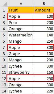
Table of Contents
1. Sum Values Based on Selection Of Drop-Down List
Step1: Copy ‘Fruit’ column to another column first. For example, column D.
Step2: On column D, click Data in ribbon, then click Remove Duplicate under Data Tools group to remove duplicate fruits from new fruit list.

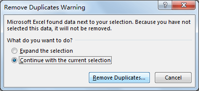
Step3: On Remove Duplicates Warning dialog, select the second option ‘Continue with the current selection’. Then click Remove Duplicates. This step makes sure you only remove the duplicate values from your new fruit list and keep the original fruit list unchanged.
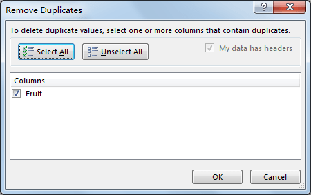
Step4: ‘Remove Duplicates’ dialog pops up. Just click OK.
Then you will notice that duplicate values are removed from column D. All fruits are unique.
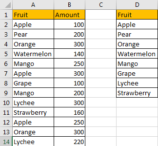
Step5: Add two new columns. See screenshot below.
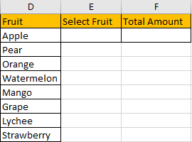
Step6: Select on E2, then click Data->Data Validation under Data Tools group.

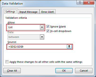
Step7: On Data Validation window. There are three tabs. Click the first ‘Settings’, select ‘List’ in Allow dropdown list; select =$D$2:$D$9 (new fruit list) in Source textbox.
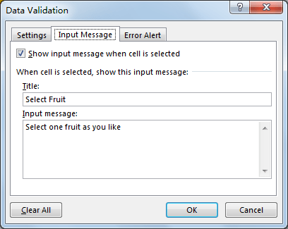
Step8: If you want to get some prompt message, you can click the second tab ‘Input Message’, and enter title and message. Then click OK.
Step9: Click on E2, verify that ‘Select Fruit’ message pops up.
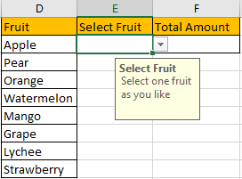
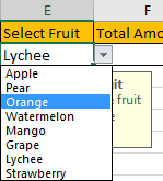
Step10: Select a fruit in dropdown list, for example ‘Orange’.
Step11: In F2, enter the formula:
=SUMPRODUCT(SUMIF($A$2:$A$14,$E$2,$B$2:$B$14))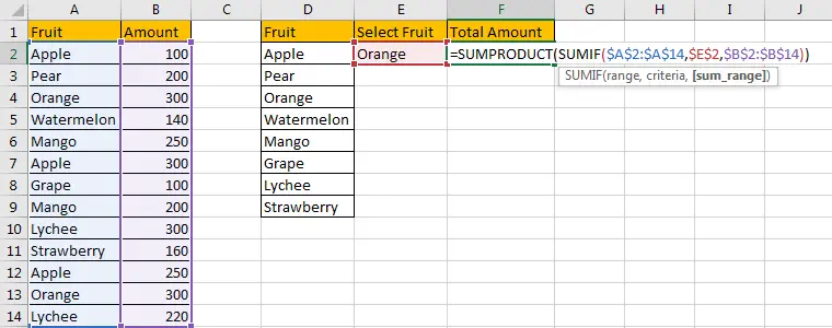
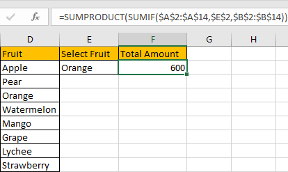
Step12: Press Enter and check the result. Verify that total amount for orange is calculated correctly.
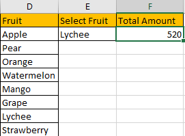
Step13: Select another fruit from dropdown menu. Verify that total amount is recalculated and updated properly.
2. Video: Sum Values Based on Selection Of Drop-Down List
This tutorial where we’ll explore a smart way to sum values based on the selection of a drop-down list in Microsoft Excel. In this video, we’ll delve into one powerful methods using data validation and Excel functions.
3. SAMPLE FIlES
Below are sample files in Microsoft Excel that you can download for reference if you wish.
4. Related Functions
- Excel SUMPRODUCT function
The Excel SUMPRODUCT function multiplies corresponding components in the given one or more arrays or ranges, and returns the sum of those products.The syntax of the SUMPRODUCT function is as below:= SUMPRODUCT (array1,[array2],…)… - Excel SUMIF Function
The Excel SUMIF function sum the numbers in the range of cells that meet a single criteria that you specify. The syntax of the SUMIF function is as below:=SUMIF (range, criteria, [sum_range])…