This post explains that how to transpose data from columns to rows, or from rows to columns in excel. if you want to rotate the data in columns of a worksheet to rearrange it in rows, you can use the “Paste Special Transpose” option to switch rows to columns or vice verse. you can also use the TRANSPOSE function to achieve the same result.
Using Paste Special Transpose
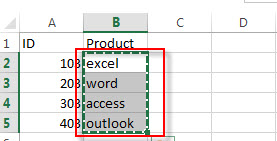
To transpose the data in the range B2:B5 from columns to rows, refer to the following steps:
1# Select the range B2:B5 that you want to rearrange, then press CTRL+C to copy the selected Range.

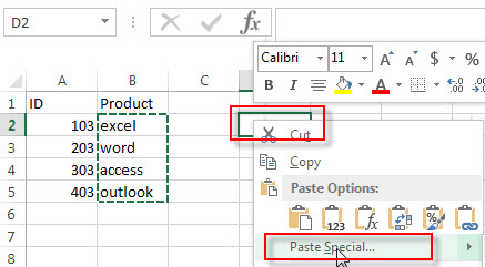
2# Select Cell D2, then Right-click on the selected range, then click “Paste Special….”, the “Paste Special” window will appear.

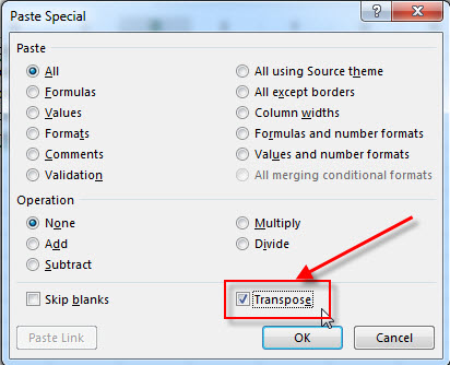
3# checked “Transpose“. click OK.

4# let’s see the last result.

Using Transpose Function
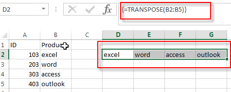
If you want to transpose the range B2:B5 to D2:G2, just enter into the following array formula in Cell C1:
=TRANSPOSE(B2:B5)
You need to select the range D2:G2, then enter the above formula in the formula bar. Then click “Ctrl”+”Shift”+Enter key to convert its as an array formula.

Related Functions
- Excel TRANSPOSE function
Excel TRANSPOSE formula allows you to rotate (swap) values from rows to columns and vice versa in Excel.The Excel TRANSPOSE Function syntax:=TRANSLATE (range) …
Leave a Reply
You must be logged in to post a comment.