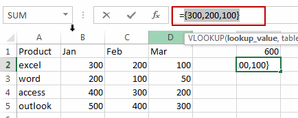
This post will guide you how to lookup a value and then return the sum of two or more related columns in Excel 2013/2016. How do I Use VLOOKUP function and SUM function to lookup a specific value and return the sum of all matches in columns in Excel.

1. Vlookup to Return the Sum of Two or More Columns

Assuming that you have a list of data in range A1:D5, in which contains sales data for three months. And you want to look up a product named “excel” in this range, and then return the sum of three months or columns. How to do it. You can use the VLOOKUP function to look up values in the given range, but the problem is that this function returns only one related sales value.  If you want the VLOOKUP function to return the values from the two or more columns, you need to put column numbers that you want returned into VLOOKUP function as its third argument.  Then the VLOOKUP function will also return an array values. Last, you can use the sum function to calculate the total value of the returned array values from VLOOKUP function.

So you can write down an Excel Array formula based on the VLOOKUP function and the SUM function as below:

=SUM(VLOOKUP("excel", A2:D5, {2,3,4}, FALSE))

Type this formula into a blank cell and press Ctrl + Shift +Enter keys on your keyboard to change it as array formula. You would notice that the total sales value of product “excel” in three months has been calculated.

Note:

• “excel” is the lookup value
• A2:D5 is the lookup range
• {2,3,4} are the column numbers that have sales values you want to return, it should be enclosed in curly braces so that to create the array of values.

Let’s see how this formula works:

= VLOOKUP(“excel”, $A$2:$D$5, {2,3,4}, FALSE)

This formula returns an array result that contain three sales values of product “excel”.

You can also use another formula based on the SUMPRODUCT and VLOOKUP functions to achieve the same result. Like this:

=SUMPRODUCT(VLOOKUP("excel", A2:D5, {2,3,4}, FALSE))

Type this formula into a blank cell and press Enter key.

The SUMPRODUCT function will return the sum of the array elements returned by the VLOOKUP Function.

2. lookup and Return the SUM of Two or More Columns using VBA

Now, let’s explore the second method, where we’ll create a VBA User Defined Function to achieve the lookup and sum operation. This approach allows for greater flexibility and customization compared to traditional formulas.

Press ALT + F11 in Excel to open the VBA editor.

In the VBA editor window, go to the “Insert” menu and select “Module.”

Copy  and paste the provided VBA code for the LookupAndSum function.

Function LookupAndSum(lookupValue As Variant, lookupRange As Range, sumRange As Range) As Double
    Dim lookupRow As Long
    Dim sumTotal As Double
    Dim i As Long
    
    ' Initialize sumTotal
    sumTotal = 0
    
    ' Loop through each cell in the lookup range
    For i = 1 To lookupRange.Rows.Count
        ' Check if the current cell matches the lookup value
        If lookupRange.Cells(i, 1).Value = lookupValue Then
            ' Get the corresponding row number
            lookupRow = lookupRange.Cells(i, 1).Row
            
            ' Loop through each cell in the sum range and add to sumTotal
            For Each cell In sumRange.Columns
                sumTotal = sumTotal + Cells(lookupRow, cell.Column).Value
            Next cell
            
            ' Exit loop after finding the first match
            Exit For
        End If
    Next i
    
    ' Return the sumTotal
    LookupAndSum = sumTotal
End Function

With this code, you can now input arguments into the LookupAndSum function.

lookupValue: The value to lookup.

lookupRange: The range where the lookup value will be searched.

sumRange: The range of columns where the sum will be calculated.

Close the VBA editor window.

Enter a formula in any cell where you want to display the sum of columns based on a lookup value.

=LookupAndSum("excel", A2:A5, B2:D5)

where “excel” is the lookup value, A2:A5 is the range to search for the lookup value, and B2:D5 is the range of columns where the sum will be calculated.

After entering the formula, press Enter to calculate and display the result.

By following these steps, you should be able to successfully run the VBA code and use the LookupAndSum function in your Excel workbook.

3. Video: lookup and Return the SUM of Two or More Columns

This Excel video tutorial, we’ll explore two methods to lookup and return the sum of two or more columns. We’ll start by utilizing an array formula combining the SUM and VLOOKUP functions, followed by creating a VBA User Defined Function.

4. Related Functions

• Excel VLOOKUP function
  The Excel VLOOKUP function lookup a value in the first column of the table and return the value in the same row based on index_num position.The syntax of the VLOOKUP function is as below:= VLOOKUP (lookup_value, table_array, column_index_num,[range_lookup])….
• Excel SUM function
  The Excel SUM function will adds all numbers in a range of cells and returns the sum of these values. You can add individual values, cell references or ranges in excel.The syntax of the SUM function is as below:= SUM(number1,[number2],…)…
• Excel SUMPRODUCT function
  The Excel SUMPRODUCT function multiplies corresponding components in the given one or more arrays or ranges, and returns the sum of those products.The syntax of the SUMPRODUCT function is as below:= SUMPRODUCT (array1,[array2],…)…