If you are an enthusiastic Google Sheets user, then you may have an urgent task to rank a specified datelist based on given multiple criteria; you can easily perform this task manually, which is also feasible, but it only works for ranking a small amount of data. However, when there are multiple pieces of data to be processed, it becomes a cumbersome and time-consuming task to sort the list of data based on multiple conditions by manually.

But don’t worry, because this article will show you how to rank with multiple criteria in google sheets.

RANK Data with Multiple Criteria

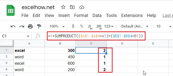
If you want to rank the specified data by just one criteria, you can use the RANK function to easily rank the values of the range of cells in google sheets. Suppose you want to rank the data of a range of cells in a worksheet with multiple criteria. So how do you accomplish that task? You need to create a new complex formula by using the SUMPRODUCT function. For example, when you want to sort the list of data in the range of cells A1:B4 by using two criteria or conditions, simply use the following formula.

=1+SUMPRODUCT(($A$1:$A$4=A1)*($B$1:$B$4>B1))

Next, you need to type this formula in the formula box in cell C1, then press Enter and drag the AutoFill handler to the other cells.

Let’s see the results.

Related Functions

• Google Sheets SUMPRODUCT function
  The Google Sheets SUMPRODUCT function multiplies corresponding components in the given one or more arrays or ranges, and returns the sum of those products.The syntax of the SUMPRODUCT function is as below:= SUMPRODUCT (array1,[array2],…)…
• Google Sheets RANK Function
  The Google Sheets Rank function is used to return the ranking of a given number from a list. If there are duplicate numbers in the list, then the numbers will be in the same rank.The syntax of the Google Sheets Rank function is explained as follows:The syntax of the Google Sheets Rank function is explained as follows:= RANK (number,reference ,[order])…