In excel worksheet, there are relative reference and absolute reference two cells set up types. Normally, relative refence is set by default. If you are not very clear about the concepts or behavior of relative reference and absolute reference, we will use below examples to illustrate them clearly and simply.
Table of Contents
Relative Reference
Case 1:
In daily work we often use formula to do calculation, and then drag the fill handle to fill other cells which want to copy the formula as well. For example, see below table, in E2 we enter the formula =B2*C2, then drag it (with formula) to fill E3 and E4, we found that in E3 the formula is automatically changed as =B3*C3.


If we move focus on E4, we may find in E4, we may find in E4 the formula is automatically updated as =B4*C4. So, in this case, Bx*Cx can be seen as relative reference. The formula is calculated properly based on the reference; it is not a fixed reference as B2*C2.
Case 2:
In above case1, the relative reference is updated properly in formula and we can get the correct result as we want. But in some cases, relative reference will cause wrong result. We use LOOKUP function here to do a demonstration.
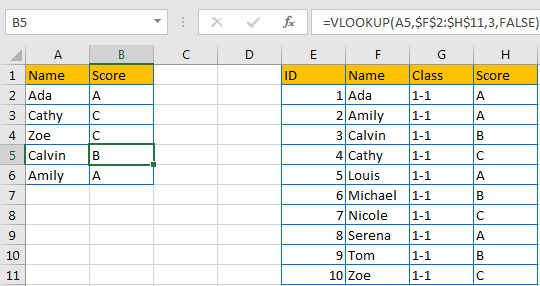
In below table, we want to get Score from table E1:H11 for person lists in A column, and record the returned value in B column accordingly, obviously we can use VLOOKUP function here.
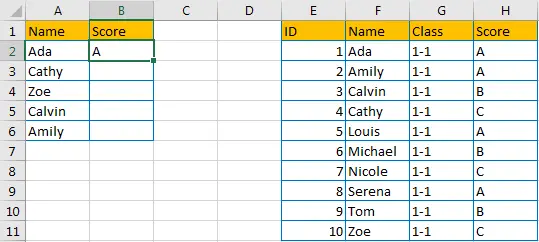
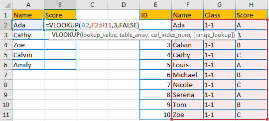
So, enter =VLOOKUP(A2,F2:H11,3,FALSE) in B2 to get result.
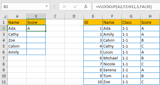
We can get the correct result A in B2 properly.
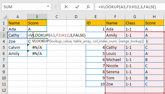
Drag the fill handle to B3:B6. Noticed that we get some wrong results.
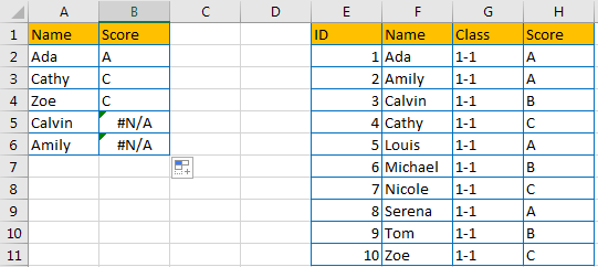
Click B2 to check the formula. Noticed that reference (for table_array) is updated to F3:H12 automatically as relative reference is set up for cells by default. In this case, Cathy still can be found in new reference, so it can return the correct score. But for Calvin, it is not included in its relative reference, so we get improper result here.
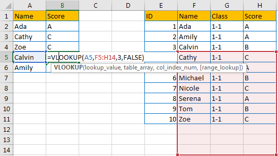
Above all, we need to keep table_array with a fixed value, so we need to know what is absolute reference here.
Absolute Reference
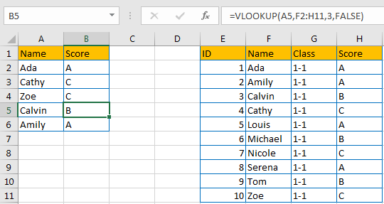
In above case2, if we keep table_array with fixed value E2:H11, then the result will be calculated correctly in column B.
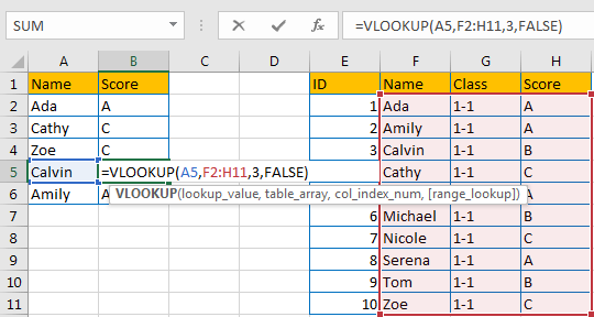
So, we can confirm that F2:H11 is absolute reference for VLOOKUP function in this case.
Change Relative Reference to Absolute Reference in Worksheet
Because relative reference is default set up in worksheet, so we just need to know how to change relative reference to absolute reference. Obviously, if we copy a cell with formula to another cell, relative reference will update automatically, if we want to use absolute reference, we have to change reference manually, it is quite troublesome. Actually, we can add $ before relative reference to change it to absolute reference, and there are two ways to implement this function, see details below.
Method 1: Add $ Manually
We still use case 2 table to do demonstration.
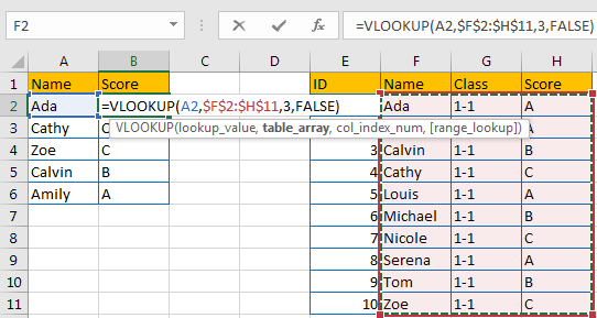
Step 1: In B2, use VLOOKUP function to search the mapping result for A2. For VLOOKUP each parameter, we can select A2 as lookup_value, select range F2:H11 as table_array directly, then enter col_index_num (in this case Score is the third column in table, so we enter 3) and select False, then click Enter to complete formula with VLOOKUP function.

Step 2: Add $ before each character of table_array.

Step 3: Drag this fill handle to fill other cells this time. Verify that $ is copied with formula to other cells as well, and F2:H11 is not changed anymore in formula after adding $.
Method 2: Add $ by Press F4
Step 1: Repeat above step#1, but this time, before clicking Enter to confirm formula, click F4 directly. You may find that $ is auto added before F2:H11 each character properly.
Change Relative Reference to Absolute Reference in Different Cases
Case 1: Add $ before Row and Number
See table below. If we want to record B2*C2, B2*C3, B2*C4 values in E2:E4 accordingly, we may add $ before B and 2 to keep B2 unchanged in formula.

Copy the cell to E3 and E4. Verify that values are calculated properly.

Case 2: Add $ before Column and Number
If we want to record B2*C2, B3*C2, B4*C2 values in E2:E4 accordingly, we may add $ before C and 2 to keep C2 unchanged in formula.

Copy the cell to E3 and E4. Verify that values are calculated properly.
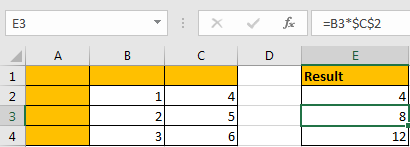
By the way, you can also add $ only before row/column depends on your requirement anyway, for example $B2:C2, B$2:C2, $B2:C$2 etc.