In daily life, we can use repeated characters to indicate the magnitude or priority of something. For example, a single “!” indicates a minor case, double “!!” indicates a medium case, and triple “!!!” indicates a high case, and so on. In an Excel worksheet, we can use REPT function to output a different number of repeated characters based on the input value to mark the difference. This approach is more convenient than creating a chart in Excel worksheet.

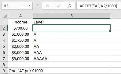
In today’s example, we want to indicate different incomes by outputting different numbers of “A” characters. Assuming the rule is one A per $1000, for example, if income is $1000, record an “A” in the “Level” column, and if income is 1750, just near 2000, but not enough for 2000, still an “A”.

Look at the following example. We use different amounts of repeated characters “A” to indicate different income levels.

In this example, you can also replace the character “A” with other characters, or even a string.

FORMULA

Excel not only contains many very useful mathematical functions, but also contains several uncommon but useful functions. REPT function is one of these uncommon functions.

Excel REPT function can output repeating characters according to the input times. It is very helpful for us to build a simple comparison with normal or special characters.

Syntax:

= REPT(text, number_times)

Example:

REPT(“*”,5) – Outputs *****

 In this example, the text is the letter “A”, character “A” should be enclosed into double quotes, and the number_times is A2/1000, depending on how many 1000s the income value contains.

The formula is:

= REPT(“A”, A2/1000)

EXPLANATION

REPT is a very simple function in Excel. We only need to confirm the output character and the number of times to output proper characters.

1.number_times Is Not an Integer & <1

In this example, the number of outputs is determined by the mathematical expression A2/1000.

A2/1000 -> Calculate repeating times

Calculate A2/1000 in Excel formula bar. The result is 0.7.

The REPT function now has two parameters confirmed, the output character is “A” and the times is “0.7”. Since times is not an integer and is less than 1, it will be truncated, so the parameter is equal to 0, no “A” is output, and an empty cell is displayed in B2.

2.number_times Is Not an Integer & >1

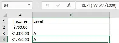
In B4, the formula is:

=REPT("A",A4/1000).

A4/1000=1.5 –> Repeating times 1.5 is not an integer, decimal part is truncated.

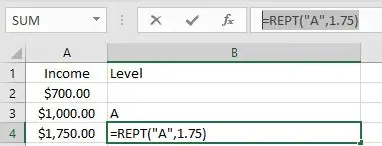
1.5 is rounded down to the nearest integer 1. So only one “A” is output and displayed in B4.

3.number_times Is an Integer

In B3, the formula is =REPT(“A”,A3/1000).

A3/1000=1 –> Repeating times is an integer

So REPT function only returns one “A”.

EXPAND

Wingdings character set and equivalent Unicode characters (alanwood.net)

Sometimes we may want to display some special characters or icons in an Excel worksheet. We can still apply the REPT function to output characters, but these special characters cannot be entered into Excel formulas because they are not accepted. At this point we need to get help from CHAR function in Excel.

CHAR function can return a character based on the entered number.

Syntax: CHAR(Number)

Depending on the font, CHAR will return different characters even if the same number is entered.

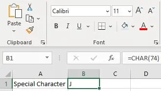
Pick font Calibri.

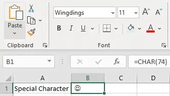
Pick font Wingdings.

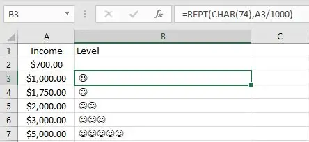
To output the smileface instead of letter “A” in the above example, we simply enter char(74) in the REPT “text” argument to replace letter “A”.

Related Functions

• Excel CHAR function
  The Excel CHAR function returns the character specified by a number (ASCII Value).The CHAR function is a build-in function in Microsoft Excel and it is categorized as a Text Function. The syntax of the CHAR function is as below:=CHAR(number)….
• Excel REPT function
  The Excel REPT function repeats a text string a specified number of times.The REPT function is a build-in function in Microsoft Excel and it is categorized as a Text Function.The syntax of the REPT function is as below:= REPT  (text, number_times)….