This post will guide you how to reverse number signs in Excel. How do I reverse the sign of a range of cells from positive to negative or negative to positive in Excel. How to reverse sign of number with a formula in Excel.

Assuming that you have a list of data in range B1:B4 that contain some numbers, and you want to reverse the sign of those numbers. You can use the below two methods to achieve it.

1. Reverse Number Signs with a Formula

You can multiply all numbers in a range of cells by a negative number 1, so that you can get the expected value. So just type the following formula in a blank cell C1.

=B1*-1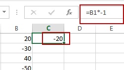

Then you need to drag the AutoFill Handle over other cells to apply this formula.

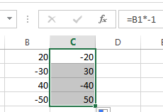
So the positive number will be converted to negative numbers and the negative number will be converted to positive numbers. Then you still need to copy and paste the last result to the original range of cells.

2. Reverse Number Signs with Paste Special Feature

You can also use the Paste Special Feature to reverse number signs in Excel. Just do the following steps:

Step1: type negative number -1 in a blank cell and press Ctrl+C to copy it.

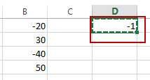
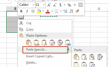
Step2: select the range of cells that contain numbers you want to reverse the signs. And right click on it and select Paste Special from the popup menu list. And the Paste Special dialog will open.

Step3: select Multiply radio button in the Operation section. And then click OK button.

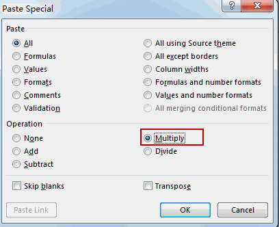
Step4: you will see that all of the selected cells will be multiplied by negative -1. And all number signs will be reversed.

3. Video: Reverse Number Signs in Excel

This video will show you how to reverse the number signs in Excel using both a formula and the Paste Special feature.