This post will guide you how to show percentages in a stacked column chart in Excel. How to display percentages as series in an Excel Stacked column chart. How to create a 100% stacked chart with percentages in Excel.

Show Percentages in a Stacked Column Chart

---

Assuming that you have a list of data in the range of cells A1:D5 contain sales data for some product. And you want to create a stacked column chart with percentages based on those data. Just do the following steps:

#1 select the original data to create a stacked column chart.

#2 go to INSERT tab, click Insert Column Chart command under charts group, and select 2-D Column from the drop down list.

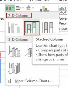
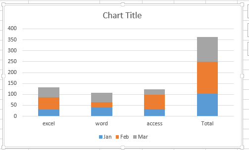
#3 a stacked column chart has been created.

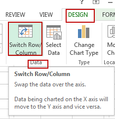
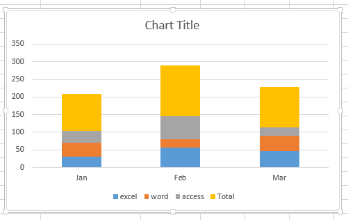
#4 go to DESIGN tab, click Switch Row/Column command under Data group.

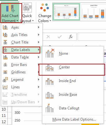
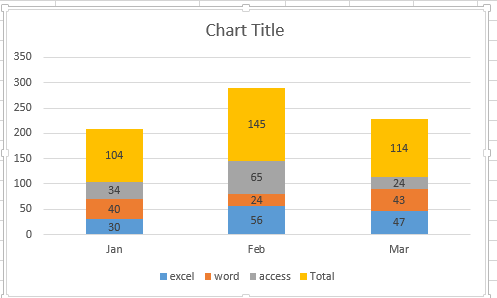
#5 go to Layout tab, click Add Chart Element command under Chart Layouts group. And then click Data Labels, select Center from the popup menu list.

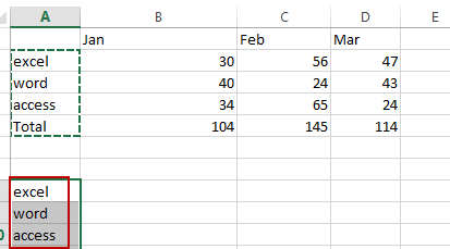
#6 select one blank range and copy all product names into it.

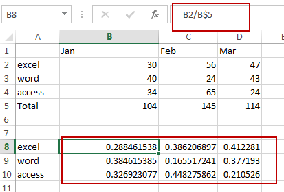
#7 you need to divide each value in the table above by the total value in the same row, so you can type the following formula into the formula box of cell B8 and then drag the fill handle over other cells to calculate the percentage values.

=B2/B$5

#8 select those decimal numbers, and then go to HOME tab, click Number format drop down list under Number group. Or directly click % icon.

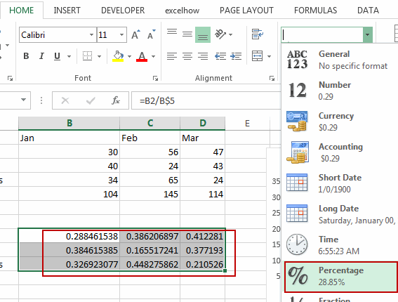
All selected numbers have been changed to percentage format.

#9 select one data label in the stacked column chart, and then type = in the formula bar, and then select percentage value, and press Enter key.

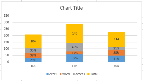
You will see that the data label has been displayed as percentage. You need to repeat this step to change other data labels.