This post will guide you how to sort the dynamic data automatically in your worksheet. How do I sort dynamic range of data with a formula in Excel.

Sort Dynamic Data

---

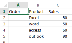
Assuming that you have a list of data in the range of cells A1:B5, if you want to sort dynamic data in your worksheet, just do the following steps:

#1 you need to insert one new column before the first column of your data. Type one name into the first cell of the new column.

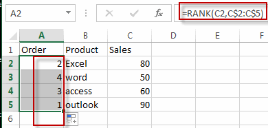
#2 type the following formula into the Cell A2 to sort sale values based on the sales column. Then press Enter key in your keyboard, and drag the AutoFill Handle over other cells A3:A5

=RANK(C2,C$2:C$5)

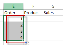
#3 select one new column, such as: Column E, and type one column name in the first cell. And select the second new column next to the column E, and type the column name as product. Then select the third new column next to the column F, type the column name as Sales in the Cell G1.

#4 insert the sequence numbers in the range of cells E2:E5

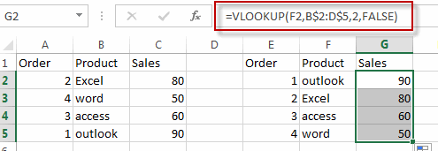
#5 type the following formula into the formula box of the cell F2, and press Enter key. Then drag the AutoFill handle over other cells F3:F5, and G2:G5.

=VLOOKUP(E2,A$2:C$5,2,FALSE)

#6 you can try to change one sale value to check if the order of product be sorted automatically in the new list of data E1:G5.

Related Functions

---

• Excel Rank function
  The Excel RANK function returns the rank of a given number in a supplied range of cells.  If there are duplicated values in a list of values, it will be set the same rank.The syntax of the RANK function is as below:= RANK (number,ref,[order])….
• Excel VLOOKUP function
  The Excel VLOOKUP function lookup a value in the first column of the table and return the value in the same row based on index_num position.The syntax of the VLOOKUP function is as below:= VLOOKUP (lookup_value, table_array, column_index_num,[range_lookup])….