In the previous post, you should know that how to fix or remove the #N/A error when using VLOOKUP formula to lookup value from another sheet. And this post will show you reasons why your VLOOKUP formula is not working in Excel 2003/2010/2013/2016 or Excel 365. You should be want to know some of the common reasons why you are getting those VLOOKUP errors, such as: #N/A, #VALUE, #REF, and returning incorrect results.
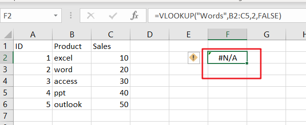
Table of Contents
Most of Common VLOOKUP Formula Errors
You should know that VLOOKUP function is a very popular and powerful used function in Microsoft Excel or Google Sheets. And most of users are also complain that the VLOOKUP function fails to work sometimes, and want to know how to fix any VLOOKUP not working problem while using VLOOKUP function to lookup value from another sheet in Excel. Let’s see some common VLOOKUP Formula errors below:
1. VLOOKUP #N/A Error
When using VLOOKUP formula to lookup one value in your table array, and if it cannot find an exact match or approximate match, then the #N/A error message would be displayed. #N/A error means “The Value is not available” in Excel. this error is the most common VLOOKUP error message while looking up values from another sheet or different sheet and returns an incorrect value.
It is not only one reason that the lookup value is not available, and there should be some reasons whey VLOOKUP formula is not working and returns errors in Excel.
#1 Lookup Value Not in the First Column
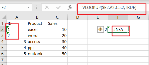
For VLOOKUP function, the Lookup value must be in the first column or the leftmost column of the table_array argument. If lookup value is not available in the first column of a table array, and the VLOOKUP formula will generate an #N/A error.
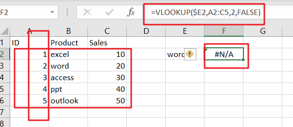
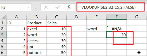
If you want to fix this VLOOKUP error in your worksheet, and you need to re-arrange your column range correctly in your table array parameter in VLOOKUP formula. for the above VLOOKUP formula example, you need to change your table_array range from A2:C5 as B2:C5 in VLOOKUP function.
#2 Using an Approximate Match
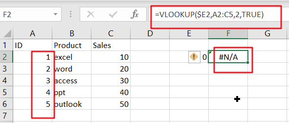
The range_lookup is an optional argument in the VLOOKUP function. And the value can be set as True or False. The default value is True. If you don’t specify this argument and Excel will assume that you want to use an approximate match. And if you want to use an Exact Match in VLOOKUP function, and you should set the fourth argument as FALSE.
Assume that the range_lookup argument is set to “FALSE” or using an approximate match in your VLOOKUP formula, if you want to lookup value from another sheet or same sheet using VLOOKUP function, and lookup value is smaller than the smallest value available in the first column of table array, and your VLOOKUP function should be generated an #N/A error.
#3 Numbers Stored or Formatted as Text
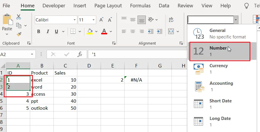
When your data is imported from an external data table or your numeric values were stored as text format, and you try to lookup a numeric value using VLOOKUP function, Excel will generate an error message #N/A.
If you want to fix this error message for VLOOKUP formula, and you have to check and format all numeric values as Number format. you can select those values, and go to “HOME” tab, and select “Number” format from the drop-down list in the Number category.
#4 Type Mistake for Lookup Value
The VLOOKUP function will use the lookup value as keyword to search for in the lookup table in your current worksheet or in another worksheet, if you mistyped the lookup value and the VLOOKUP function will not find what you typed and Excel will return you an error message #N/A.
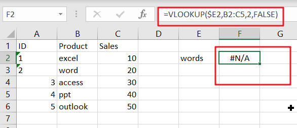
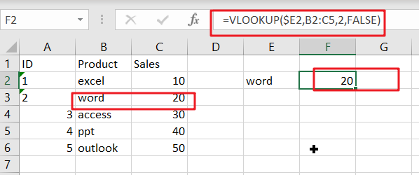
For example, if you want to type the lookup value “word”, but mistyped as “words”, and the VLOOKUP function would display the #N/A error message. When the keyword was typed correctly, and the formula should be able to find the expected value.
#5 Extra Space or Characters (Leading and trailing spaces for Lookup value)
If the lookup value contains extra space or characters in the formula, and the VLOOKUP function will also generate an error message #N/A. the #N/A error is caused by extra spaces which your eyes can hardly see, and everything looks good.
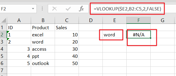
To fix or remove this error, and you should check for extra spaces in the formula or remove leading and trailing spaces in the lookup value using TRIM function.
2. VLOOKUP #REF error
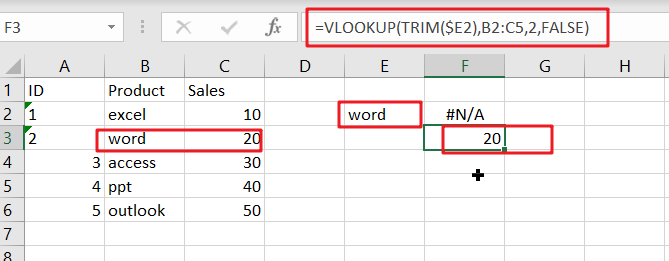
#1 Count the Wrong column number for Column_index_num parameter
If you count the wrong column number for Column index number parameter in the third argument of the VLOOKUP function, and it will also generate an error message #N/A. To fix this error, you need to recount the COLUMNS count from the table array that you are getting your data in your VLOOKUP formula.
3. VLOOKUP #VALUE Error
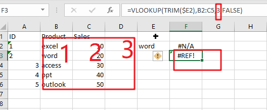
If you enter wrong data type in the VLOOKUP formula in Excel, and the #VALUE error will generate. And the below reasons will also cause this error.
- Index Number is less than 1
If your Index_number argument is less than 1 in VLOOKUP function, and it will return a #VALUE error.
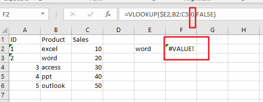
- Lookup Value Length
You need to know that lookup value length should not be exceeded 256 characters, if lookup value character length exceeds this limit in VLOOKUP formula, and it returns a #VALUE error.
To fix this error, you can use INDEX function in combination with MATCH function to build another newly formula to achieve the same request.
4. Removing VLOOKUP Error Messages
If you want to make VLOOKUP errors clearer and easier to understand, and you can use the IFERROR function to display a meaningful message if VLOOKUP is not working and returns error.
=IFERROR(VLOOKUP($E2,Sheet8!B2:C5,2,FALSE),"lookup value not found!!!")
The IFERROR function can be used to check for any errors in the VLOOKUP formula, and if one VLOOKUP error message is returned by the VLOOKUP formula, excel will display “lookup value not found!!!” instead of any of the error messages, such as: #N/A,#REF,and #VALUE.

Enjoy!
Related Functions
- Excel IFERROR function
The Excel IFERROR function returns an alternate value you specify if a formula results in an error, or returns the result of the formula.The syntax of the IFERROR function is as below:= IFERROR (value, value_if_error)…. - Excel VLOOKUP function
The Excel VLOOKUP function lookup a value in the first column of the table and return the value in the same row based on index_num position.The syntax of the VLOOKUP function is as below:= VLOOKUP (lookup_value, table_array, column_index_num,[range_lookup])…. - Excel INDEX function
The Excel INDEX function returns a value from a table based on the index (row number and column number)The INDEX function is a build-in function in Microsoft Excel and it is categorized as a Lookup and Reference Function.The syntax of the INDEX function is as below:= INDEX (array, row_num,[column_num])… - Excel MATCH function
The Excel MATCH function search a value in an array and returns the position of that item.The MATCH function is a build-in function in Microsoft Excel and it is categorized as a Lookup and Reference Function.The syntax of the MATCH function is as below:= MATCH (lookup_value, lookup_array, [match_type])….